Announcements
This section describes the format of and some features associated with GNIRS data. More detailed information on reduction of GNIRS data accompanies the GNIRS IRAF package. GNIRS imaging can be reduced with the DRAGONS data reduction software.
- CLEANIR
- Reducing XD spectra (see below)
- Gemini IRAF package
- To browse what Gemini Users have exchanged about tricks, issues and solutions regarding reduction of GNIRS data, please go to the DR forum (tag=GNIRS).
Reducing XD spectra
This web page goes through the steps involved in reducing GNIRS cross-dispersed (XD) spectra using the Gemini IRAF package (v1.13.1). These spectra of a nearby galaxy nucleus were taken with the short (0.15 arcsec/pix) blue camera and 32 l/mm grating, the most commonly-used XD mode, but the data reduction steps will be broadly applicable to data taken in other XD configurations as well. The IRAF tasks can be used in several different ways according to the characteristics of the specific data set and the user's personal preference. The procedure shown here will not be optimal for all XD observations, but is intended as a starting point for those new to GNIRS data.
For more information about GNIRS data reduction and how the tasks can be used, try the following:
- General GNIRS data reduction information: type "gnirsinfo" on the IRAF command line after loading the Gemini and GNIRS packages (also at this web page)
- Information about XD reductions: type "gnirsinfoxd" (also linked from this web page; gnirsinfols and gnirsinfoifu also available)
- Example reduction scripts: type "gnirsexamples"
- Help pages for individual tasks
- Published science papers based on GNIRS data, e.g. Kriek et al. (2006), Burleigh et al. (2006)
- This ADASS paper is several years old but may be useful for general background information
- Various general near-IR data reduction tutorials are available on the web
- Problems can be reported through the helpdesk
- An alternative way to reduce the GNIRS cross-dispersed mode data is using PypeIt.
The steps discussed on this page are:
- Inspecting and sorting the data
- Pattern noise cleaning
- Dealing with radiation events in short camera data
- Preparing the data reduction environment
- "Preparing" the data
- Making the flatfield
- Reducing the science data
- Wavelength calibration and s-distortion correction
- Extracting spectra
- Telluric line cancellation and flux calibration
Sorting/inspecting the data
We will be working on data taken for GN-2011A-Q-126, a poor weather program designed to make use of the telescope in cloudy conditions. Usually the PI will download their data from the Gemini Observatory Archive (see this page for some help with using the archive). If you are not the PI of the program, this retrieval option is available after the proprietary period of the data has ended. Files retrieved from the archive may contain various types of data, depending on the search method: acquisition images, calibration data, science target spectroscopy, etc. Before starting the reduction, we need to work out which files are which. There at least three ways of doing this, and it can be helpful to combine a couple of them to get a good sense of the data. Note that the first method currently only works if you are the PI of the program such that you have access to the program in the OT.
- Use the OT to fetch and inspect the program (PI of the program only) :

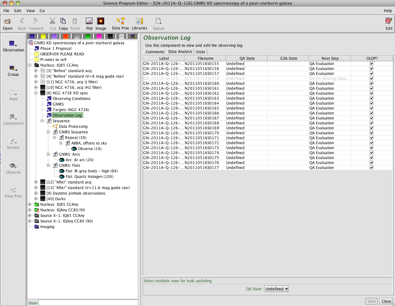
- As observations in an observing programme are executed, their colour changes to reflect their status. Green, "ready" observations change to black on completion, so the above left screenshot shows that the acquisition and spectroscopy of NGC 4736 in the "Nucleus: IQ85 CCAny" group has been observed, along with a telluric standard and some daytime calibrations. The grey, "inactive" observations are no longer relevant and will not be scheduled.
- The shaded steps in the "Sequence" view are those that have been completed. In this case, the first ABBA was executed, then the observer skipped ahead to take the flats and arcs and then move onto another programme as the weather was improving enough to allow regular queue observations.
- The righthand screenshot shows the "Observation Log". This gives the filenames associated with the individual steps and also the "QA State". The QA state can be "Pass" (no known problems that would make the observations unsuitable for the intended science use), "Usable" (problems such as violation of the requested observing condition constraints, but possibly useful anyway), "Fail" (fatally compromised) or "Undefined". As Q126 was a low-priority, band 4 "filler" programme, no quality assessment has been performed and all the QA states are undefined. Clicking on the "Comments" tab would show any comments left by the observer as they acquired the data (also given in the obslog, below). - Use the observing log downloaded from the archive along with the data:
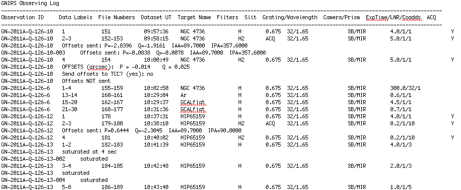
This extract gives a chronological record of the observations, showing the observer's comments as well as file numbers and details of the instrument configuration, object being observed, etc. In this case we can see that the observer recorded the offsets used to centre the galaxy and telluric standard in the slit, and also noticed that the initial standard star spectra were saturated and reduced the exposure time to compensate.
- Use the file headers. For example:
ecl> hselect N20110516*[0] field=$I,OBJECT,OBSTYPE,OBSCLASS expr=yes
N20110516S0151.fits[0]  "NGC 4736"      OBJECT  acq
N20110516S0152.fits[0]  "NGC 4736"      OBJECT  acq
N20110516S0153.fits[0]  "NGC 4736"      OBJECT  acq
N20110516S0154.fits[0]  "NGC 4736"      OBJECT  acq
N20110516S0155.fits[0]  "NGC 4736"      OBJECT  science
N20110516S0156.fits[0]  "NGC 4736"      OBJECT  science
N20110516S0157.fits[0]  "NGC 4736"      OBJECT  science
N20110516S0159.fits[0]  "NGC 4736"      OBJECT  science
N20110516S0160.fits[0]  Ar      ARC     partnerCal
N20110516S0161.fits[0]  Ar      ARC     partnerCal
N20110516S0162.fits[0]  GCALflat        FLAT    partnerCal
N20110516S0163.fits[0]  GCALflat        FLAT    partnerCal
N20110516S0164.fits[0]  GCALflat        FLAT    partnerCal
N20110516S0165.fits[0]  GCALflat        FLAT    partnerCal
N20110516S0166.fits[0]  GCALflat        FLAT    partnerCal
N20110516S0167.fits[0]  GCALflat        FLAT    partnerCal
N20110516S0168.fits[0]  GCALflat        FLAT    partnerCal
N20110516S0169.fits[0]  GCALflat        FLAT    partnerCal
N20110516S0170.fits[0]  GCALflat        FLAT    partnerCal
N20110516S0171.fits[0]  GCALflat        FLAT    partnerCal
N20110516S0172.fits[0]  GCALflat        FLAT    partnerCal
N20110516S0173.fits[0]  GCALflat        FLAT    partnerCal
N20110516S0174.fits[0]  GCALflat        FLAT    partnerCal
N20110516S0175.fits[0]  GCALflat        FLAT    partnerCal
N20110516S0176.fits[0]  GCALflat        FLAT    partnerCal
N20110516S0177.fits[0]  GCALflat        FLAT    partnerCal
N20110516S0178.fits[0]  HIP65159        OBJECT  acqCal
N20110516S0179.fits[0]  HIP65159        OBJECT  acqCal
N20110516S0180.fits[0]  HIP65159        OBJECT  acqCal
N20110516S0181.fits[0]  HIP65159        OBJECT  acqCal
N20110516S0182.fits[0]  HIP65159        OBJECT  partnerCal
N20110516S0183.fits[0]  HIP65159        OBJECT  partnerCal
N20110516S0184.fits[0]  HIP65159        OBJECT  partnerCal
N20110516S0185.fits[0]  HIP65159        OBJECT  partnerCal
N20110516S0186.fits[0]  HIP65159        OBJECT  partnerCal
N20110516S0187.fits[0]  HIP65159        OBJECT  partnerCal
N20110516S0188.fits[0]  HIP65159        OBJECT  partnerCal
N20110516S0189.fits[0]  HIP65159        OBJECT  partnerCal
N20110516S0379.fits[0]  GCALflat        FLAT    dayCal
N20110516S0380.fits[0]  GCALflat        FLAT    dayCal
N20110516S0381.fits[0]  GCALflat        FLAT    dayCal
N20110516S0382.fits[0]  GCALflat        FLAT    dayCal
N20110516S0383.fits[0]  GCALflat        FLAT    dayCal
N20110516S0408.fits[0]  Dark    DARK    dayCal
N20110516S0409.fits[0]  Dark    DARK    dayCal
N20110516S0410.fits[0]  Dark    DARK    dayCal
N20110516S0411.fits[0]  Dark    DARK    dayCal
N20110516S0412.fits[0]  Dark    DARK    dayCal
N20110516S0413.fits[0]  Dark    DARK    dayCal
N20110516S0414.fits[0]  Dark    DARK    dayCal
N20110516S0415.fits[0]  Dark    DARK    dayCal
N20110516S0416.fits[0]  Dark    DARK    dayCal
N20110516S0417.fits[0]  Dark    DARK    dayCal
Evidently the galaxy was acquired and then four spectra were taken. These were followed by arcs and flats, then a telluric standard was acquired and observed. More flats were taken the morning after the nighttime observations, along with a set of darks. (The darks were taken for test purposes and are not necessary for the reduction.) Note that comments from the observer or QA staff are not recorded in the headers, although the QA states are.
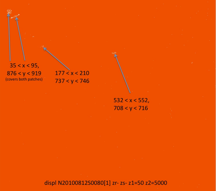
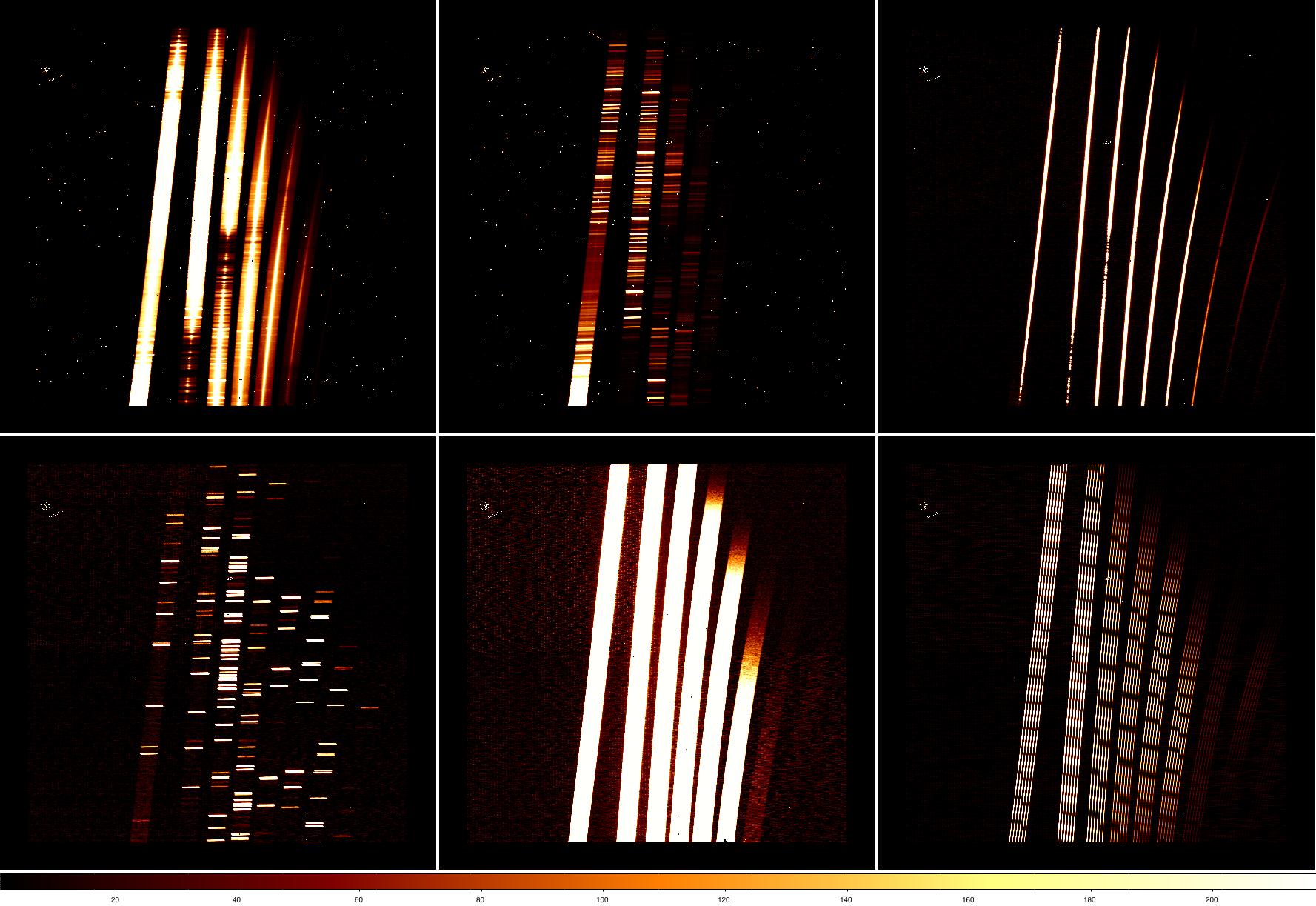
Of course, it's always a good idea to look at each of the files and measure some statistics before starting to reduce the data. The figure below shows some of the data taken for this program (we'll take a look at the statistics in the next section). Clockwise from top left:
- XD spectrum of the galaxy nucleus, with emission filling the short slit. The leftmost order (order 3) roughly corresponds to the K band, with the other orders covering progressively shorter wavelengths. Wavelength increases from top to bottom in the raw data. Other features visible in the data (click on the figure for a larger view) include radiation events (which look like cosmic ray hits) from the short camera lenses and a few patches of bad pixels. A close look also shows faint vertical striping.
- One of the sky frames. As the above OT screenshot shows, the data were taken in an ABBA pattern nodding to blank sky 50 arcsec from the extended galaxy nucleus. The faint "spectrum" in the blank sky frame is actually low-level persistence from the bright galaxy in the previous exposure.
- One of the telluric standard star spectra. As the exposures are much shorter (1 sec vs 300 sec), sky lines and radiation events are not obvious in the image.
- Daytime pinhole flat, used for tracing the spectra.
- Nighttime flat taken with the Quartz Halogen lamp. Flats taken with the IR lamp look similar but only have strong emission in order 3 (~K band, leftmost order).
- Argon arc spectrum
Pattern noise cleaning
GNIRS spectra are frequently affected by striping caused by the detector controller. This can usually be effectively removed using the cleanir.py script (a standalone python script, not part of the IRAF package) either at the start of the reduction or after running nsprepare. The vertical pattern is not prominent in this particular data set, however, and running the cleanir.py script has little effect. If we were to use it, the syntax would be something like this (run outside IRAF):
cleanir.py N20110516S0155.fits
See the cleanir github repo for more details. The nvnoise task in the GNIRS IRAF package is also available for modelling and subtracting electronic striping; type "help nvnoise" for details. The user is advised to visually inspect the cleaned files output by cleanir.py/nvnoise before proceeding with the rest of the reduction.
Dealing with radiation events in short camera data
Before 2012B, GNIRS spectra taken with the short cameras are affected by radiation events from the radioactive short camera lens coatings. A number of these can be seen in the galaxy spectra shown above. The radiation events, which bear some resemblance to cosmic ray hits, can be dealt with in several ways depending on the characteristics of the data. For example:
- Cosmic ray detection algorithms (e.g. IRAF's crutil package) can be used to detect and remove the radiation events
- Most tasks outside the Gemini IRAF package do not automatically preserve the Multi-Extension Fits (MEF) structure needed by the package. The fitsutil package provides tasks that can be used to manipulate MEF files
- Masks generated by cosmic ray detection algorithms can be passed to nsprepare using the "bpm" parameter, causing them to be written into the prepared file's DQ array
- The affected pixels can later be masked using nscombine's "masktype" and "maskvalue" parameters
- When run with fl_nonlinear+ and fl_sat+ (the default), nsprepare will add most of the affected pixels to the DQ array in any case
- Setting the fl_cravg flag in nsprepare causes the task to attempt to identify radiation events in each file
- These are added to the data quality array and can be removed later in the data reduction
- Pixel rejection algorithms can be employed when combining files
- In some circumstances the radiation events can simply be ignored
- For instance, affected pixels in arc spectra may have little effect on the data reduction, depending on which columns are used for the wavelength calibration
- The user could identify and interpolate over spikes in the extracted, 1D spectra
For the calibration data we will use option (4). The same could also be tried with the science data. However with this particular data set we only have two files at each nod position, so the data aren't well-suited to the use of sigma-clipping algorithms. Some experimentation shows that (3) doesn't give good results for this data set, so we will instead use a version of option (1) later in the reduction.
Preparing the data reduction environment
Before starting to reduce the data we need to load the necessary IRAF packages, define various files and make some data lists. First, we load the gemini and gnirs packages and make sure the right defaults are set. If using IRAF:
ecl> gemini
ecl> gnirs
If using PyRAF:
--> from pyraf.iraf import gemini
--> from pyraf.iraf import gnirs
Then:
ecl> unlearn gemini
ecl> unlearn gemtools
ecl> unlearn gnirs
Optionally, we can define a database directory and log file to be used for this specific pass through this particular data set. If these are not set, the default is to use a "database" subdirectory in the working directory and to write the task output to a file named "gnirs.log".
ecl> gnirs.logfile = "Q126.log"
ecl> gnirs.database = "Q126_database"
If desired, separate paths to the raw and calibration data can also be defined (see e.g. gnirsexamples GN-XD-SCI for more information). For this reduction, however, we will simply do everything in the current working directory.
Before we create the data lists, a word on the XD flatfields. For reasons that are explained below, two sets of nighttime flats are taken using different lamps. The flats taken during the day are generally pinhole flats. These flats need to be processed separately, so we need to find out which belong to which set:
ecl> hselect N20110516*[0] field=$I,GCALLAMP,SLIT expr='OBSTYPE=="FLAT"'
N20110516S0162.fits[0]  IRhigh  0.68arcsec_G5530
N20110516S0163.fits[0]  IRhigh  0.68arcsec_G5530
N20110516S0164.fits[0]  IRhigh  0.68arcsec_G5530
N20110516S0165.fits[0]  IRhigh  0.68arcsec_G5530
N20110516S0166.fits[0]  IRhigh  0.68arcsec_G5530
N20110516S0167.fits[0]  IRhigh  0.68arcsec_G5530
N20110516S0168.fits[0]  QH      0.68arcsec_G5530
N20110516S0169.fits[0]  QH      0.68arcsec_G5530
N20110516S0170.fits[0]  QH      0.68arcsec_G5530
N20110516S0171.fits[0]  QH      0.68arcsec_G5530
N20110516S0172.fits[0]  QH      0.68arcsec_G5530
N20110516S0173.fits[0]  QH      0.68arcsec_G5530
N20110516S0174.fits[0]  QH      0.68arcsec_G5530
N20110516S0175.fits[0]  QH      0.68arcsec_G5530
N20110516S0176.fits[0]  QH      0.68arcsec_G5530
N20110516S0177.fits[0]  QH      0.68arcsec_G5530
N20110516S0379.fits[0]  QH      LgPinholes_G5530
N20110516S0380.fits[0]  QH      LgPinholes_G5530
N20110516S0381.fits[0]  QH      LgPinholes_G5530
N20110516S0382.fits[0]  QH      LgPinholes_G5530
N20110516S0383.fits[0]  QH      LgPinholes_G5530
So, we have six flats taken with the IR lamp, 10 with the QH lamp, and five daytime pinhole flats. We can now delete any existing list files and construct lists containing the various kinds of data. As we already know (from inspecting the OT and observing log, above) that some of the standard star spectra were saturated, we only include the good data in telluric.lis (we can also check the observer's judgment using the nsprepare task, later).
ecl> delete *.lis ver- >& dev$null
ecl> gemlist N20110516S 155-157,159 > obj.lis
ecl> gemlist N20110516S 160-161 > arcs.lis
ecl> gemlist N20110516S 162-167 > IRflats.lis
ecl> gemlist N20110516S 168-177 > QHflats.lis
ecl> gemlist N20110516S 186-189 > telluric.lis
ecl> gemlist N20110516S 379-383 > pinholes.lis
ecl> concat arcs.lis,QHflats.lis,IRflats.lis,pinholes.lis > cals.lis
ecl> concat obj.lis,telluric.lis,cals.lis > all.lis
This is also a good time to measure some statistics on the files, record them in the log file and check for obviously deviant files that may have slipped past our earlier visual inspection and need to be excluded from the reduction:
ecl> printlog "--------" Q126.log verbose+
ecl> delete tmpfiles verify- >& dev$null
ecl> gemextn @all.lis process="expand" index="1" > tmpfiles
ecl> printlog "Image statistics"  Q126.log ver+
ecl> imstatistic @tmpfiles | tee (gnirs.log, append+)
ecl> delete tmpfiles
Finally, we use the nsheaders command to set the header keywords to be used by subsequent tasks:
ecl> nsheaders gnirs
The call to nsheaders must be repeated each time IRAF/PyRAF is restarted and the gnirs package loaded. If this is not done, each task will give the following kind of prompt:
ecl> nsprepare
Input GNIRS image(s):
Name of science extension:
Name of variance extension:
Name of data quality extension:
Header keyword for digital averages:
Header keyword for number of co-adds:
etc.
Preparing the data
At this point we can start preparing the data for further reduction. The nsprepare task (type "help nsprepare") can perform various operations such as adding variance and data quality extensions and attaching the mask definition file (MDF) to the data. The MDF gives the location of each order on the detector, so that the orders can eventually be "cut" and written into separate file extensions. The MDFs were defined during commissioning and are supplied with the Gemini IRAF package (in the gnirs$data directory). However, the exact location of the orders can change from observation to observation because of, for example, the inexact repeatability of the prism turret, deliberate recalibrations of the prism turret, or flexure. By setting shiftx=INDEF, shifty=INDEF and obstype=FLAT, we make the nsprepare task use the first flatfield in the input list to measure the location of the orders with respect to the pre-defined MDF. With the default parameter settings, the task will also check and attempt to correct the world coordinate system, flag saturated pixels and add variance and data quality extensions. At the time of writing we do not recommend using the nonlinearity correction provided by nsprepare on data taken with GNIRS at Gemini North, so we disable the fl_correct flag. A table in the gnirs$data directory, "array.fits" is used by nsprepare to obtain information about saturation levels etc.
ecl> imdelete n@all.lis verify- >& dev$null
ecl> nsprepare @all.lis shiftx=INDEF shifty=INDEF obstype=FLAT fl_correct-
arraytable="gnirs$data/array.fits"
.
.
NSPREPARE: Will measure MDF offset using N20110516S0162
NSOFFSET: Integer offset for gnirs$data/gnirsn-sxd-short-32-mdf is 36.
NSOFFSET: Final offset for gnirs$data/gnirsn-sxd-short-32-mdf is 36.0.
NSOFFSET: Shifting gnirsn-sxd-short-32-mdf-1508_12.fits[1] in X by 36.0 pixels.
.
.
The files output by nsprepare look the same as the original files but now include extensions containing the MDF, science data, and variance and data quality arrays. The gemextn or fxhead tasks can be used to compare the structure of the files before and after running nsprepare:
ecl> fxhead N20110516S0168
EXT#  EXTTYPE             EXTNAME      EXTVE DIMENS      BITPI INH OBJECT
0     N20110516S0168.fits                                16        GCALflat
1     IMAGE                            -1    1024x1022   -32
ecl> fxhead nN20110516S0168
EXT#  EXTTYPE             EXTNAME       EXTVE DIMENS     BITPI INH OBJECT
0     nN20110516S0168.fit                                16        GCALflat
1     BINTABLE            MDF                 72x6       8
2     IMAGE               SCI           1     1024x1022  -32   F   GCALflat
3     IMAGE               VAR           1     1024x1022  -32   F   GCALflat
4     IMAGE               DQ            1     1024x1022  16    F   GCALflat
It can be useful to look at the DQ extensions of the files. In the figure below, we can see that nsprepare has identified some of the pixels in the galaxy spectrum in orders 3 and 4 in file 159 as nonlinear. This is quite correct; as the clouds cleared during the observation, the bright galaxy rose above the nonlinear limit of approx. 5500ADU. This nonlinear "limit" is well below the actual saturation level of ~7500 ADU and has been set conservatively based on the properties of the detector's odd-even effect, to ensure that that effect can be removed during the data reduction. As the counts in the galaxy only slightly exceed that limit, we will not exclude that file from this training data set.
A number of pixels corresponding to radiation events have also been flagged in the DQ array (see #2 above), as have the known bad pixel patches.

Making the flatfield
Before creating the master flatfield we need to "cut" the individual flat files so that each order is written into a separate extension, as described in the previous section. We will also cut the arcs and pinholes for use later in the reduction. We use the nsreduce task for this (nscut could also be used; type "help nsreduce" or "help nscut"). Setting section="" in the call to nsreduce makes the task cut the data according to the sections defined in the MDF.
ecl> imdelete rn@cals.lis verify- >& dev$null
ecl> nsreduce n@cals.lis fl_sky- fl_cut+ section="" fl_flat- fl_dark- fl_nsappwave-
fl_corner+
The cut data have the following file format, with the science data for order 3 in extension [SCI,1], order 4 in [SCI,2], etc. Again, gemextn or fxhead can be used to see the file structure:
ecl> gemextn rnN20110516S0168
rnN20110516S0168[0]
rnN20110516S0168[1][MDF]
rnN20110516S0168[2][SCI,1]
rnN20110516S0168[3][VAR,1]
rnN20110516S0168[4][DQ,1]
rnN20110516S0168[5][SCI,2]
rnN20110516S0168[6][VAR,2]
rnN20110516S0168[7][DQ,2]
rnN20110516S0168[8][SCI,3]
rnN20110516S0168[9][VAR,3]
rnN20110516S0168[10][DQ,3]
rnN20110516S0168[11][SCI,4]
rnN20110516S0168[12][VAR,4]
rnN20110516S0168[13][DQ,4]
rnN20110516S0168[14][SCI,5]
rnN20110516S0168[15][VAR,5]
rnN20110516S0168[16][DQ,5]
rnN20110516S0168[17][SCI,6]
rnN20110516S0168[18][VAR,6]
rnN20110516S0168[19][DQ,6]
At this stage it is a good idea to check that the orders have been properly cut. This can be done using a single call to the nxdisplay task, or just by displaying each science extension in turn:
ecl> nxdisplay rnN20110516S0168 fr=1
ecl> display rnN20110516S0168[SCI,1] fr=1
ecl> display rnN20110516S0168[SCI,2] fr=1
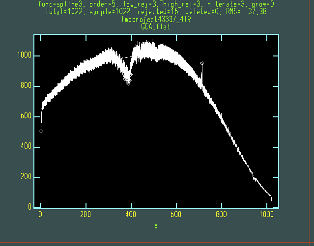
...etc. The image below shows order 5 (extension SCI,3) in one of the QH flats cut using the shifted MDF obtained above (left) and the original, unshifted MDF (right). As in the left-hand image, the whole length of the slit (approx 47 pix for the 0.15 arcsec/pixel camera) should be visible and only one order included in the cut data. If the image looked more like the one on the right, we would start troubleshooting by checking the settings in nsprepare and inspecting the flat used for the cross-correlation.
Before making the flat, it can be useful to examine the image statistics for the individual flatfield exposures to look for abnormal count levels or unusually high standard deviations that may indicate data that should be excluded from the final flat. For example, these commands run imstat on some orders of the reduced flats and print the results to the logfile we defined earlier:
ecl> printlog "--------" Q126.log verbose+
ecl> delete tmpflat
ecl> gemextn rn@IRflats.lis process="expand" extname="SCI" extver="1" > tmpflat
ecl> printlog "IR order 3 Flats"  Q126.log verbose+
ecl> imstatistic @tmpflat | tee (gnirs.log, append+)
ecl> delete tmpflat
ecl> gemextn rn@QHflats.lis process="expand" extname="SCI" extver="2" > tmpflat
ecl> printlog "QH order 4 Flats"  Q126.log verbose+
ecl> imstatistic @tmpflat | tee (gnirs.log, append+)
ecl> delete tmpflat
... and similarly for the other orders. As explained below, only order 3 (extension [SCI,1]) of the IR flats and orders 4-8 ([SCI,2] - [SCI,6]) of the QH flats are relevant.
We now use the nsflat task (type "help nsflat") to construct two sets of flats. The IR flats are used for order 3, and the QH flats for the higher orders. This is because the QH lamp contains a strong spectral feature in the K band which can only be fit by a spline of very high order. If for some reason IR flats are not available or the user does not wish to use them, the QH lamp can be used with a low-order fit but the flatfielded spectra will contain a prominent artefact in order 3 until divided by the (flatfielded) telluric standard. Both lamps have other spectral features but they are weaker and can be fit by a lower-order spline and/or can be ignored.
The short exposure times used for the flats (typically just a few seconds at low-moderate spectral resolution) mean that they are affected by few radiation events. By default nsflat applies a pixel rejection algorithm which can be tuned to screen out such deviant pixels (see the "rejtype" and associated parameters). Alternatively, images in which radiation events are identified in the DQ array added by nsprepare can be excluded from the files used to create the flat. For this example, it is not necessary to reject any pixels/files because of radiation events.
It is not usually necessary to run nsflat interactively on the IR flats (although it never hurts to do so, at least initially), but it can be a good idea to check the fitting of the QH flats interactively. As the IR flat is only used for order 3 there is little signal in the higher orders, and the warnings given by nsflat about those orders can be ignored.
ecl> imdelete IRflat,IRflat_bpm.pl verify- >& dev$null
ecl> nsflat rn@IRflats.lis flatfile="IRflat.fits" fl_corner+ process="fit" order=10
lthresh=100. thr_flo=0.35 thr_fup=1.5
ecl> imdelete QHflat,QHflat_bpm.pl verify- >& dev$null
ecl> nsflat rn@QHflats.lis flatfile="QHflat.fits" fl_corner+ process="fit" order=5
lthresh=50. thr_flo=0.35 thr_fup=4.0 fl_inter+
When run interactively, nsflat should show a fairly smooth and well-fit curve for each of orders 4 - 8 of the QH flat (below). The higher orders only have signal over a portion of the array, and order 3 can be ignored as it is not used in the final flatfield (just hit "q" to continue to the next order). The fit order can be adjusted by typing ":order 8" (for example) in the plot window, and then "f" to redo the fit; hit "?" on the plot window for more options. The "fuzz" in the fitted data is due to the "odd-even effect". This is present in all data from GNIRS at Gemini North and will have divided out by the end of the reduction.
We now need to combine order 3 of the IR flat with orders 4-8 of the QH flat. For this to work as shown below, the data format must be as shown above (this should come automatically out of the above reduction steps). To combine the normalised IR and QH flats into a single master flat:
ecl> imdelete final_flat.fits verify- >& dev$null
ecl> fxcopy IRflat.fits final_flat.fits "0-3" new_file+
ecl> fxinsert QHflat.fits final_flat.fits[3] groups="4-18"
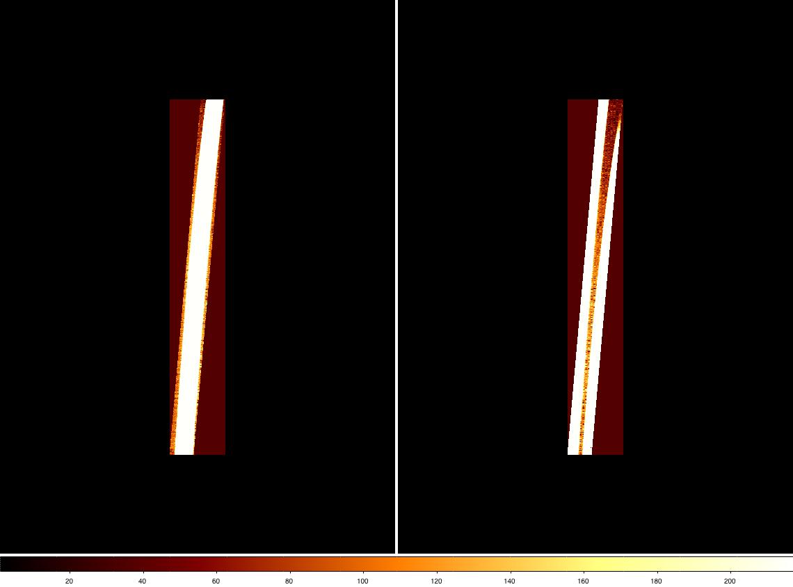
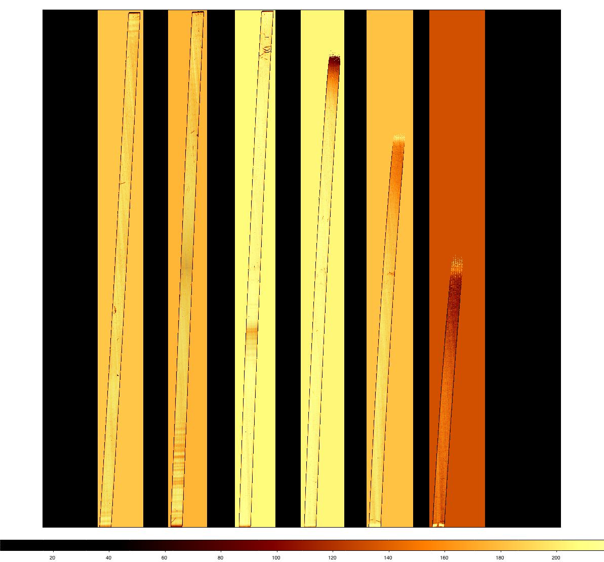
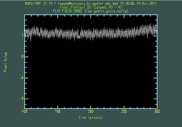
The final flat from this process is shown below, using nxdisplay. Some features are visible, such as the dark "scratches" at the top of order 5. These are genuine features of the detector and have been there since the array was received. A vertical cut through a portion of the flat shows it to be well-normalised, and the "odd-even effect" is present at about the 10% level.
Reducing the science data
We start by cleaning the science data of radiation events. As discussed above, if we had several images per offset position we could construct median images to detect and replace the events, or take advantage of one of the pixel rejection algorithms in nscombine or nsstack (below). With just two images at each offset position, though, we will try the following:
Create a relatively clean comparison frame using the minimum of the two images at each position:
ecl> imdel min155,min156
ecl> gemcombine nN20110516S0155,nN20110516S0159 output=min155 combine=median
reject=minmax nhigh=1 nlow=0
ecl> gemcombine nN20110516S0156,nN20110516S0157 output=min156 combine=median
reject=minmax nhigh=1 nlow=0
Estimate the noise at that pixel using the RDNOISE and GAIN header keywords (written into the headers by nsprepare), and identify pixels deviating by some amount above the noise in the minimum frame. These spectra were taken through variable cloud cover and therefore have rather different flux levels, so the thresholds used in imexpr are not the same for all files. Some experimentation was needed to find thresholds that effectively identified radiation events with few or no false positives at the location of the galaxy spectrum or at the edges of the spectral orders:
ecl> hselect n@obj.lis field=$I,RDNOISE,GAIN expr=yes
nN20110516S0155 6.19    13.50
...
ecl> imdel mask15?.pl
ecl> imexpr expr= "(a-b)>30*sqrt(6.19**2+2*b/13.50) ? 1 : 0" output=mask155.pl
a=nN20110516S0155.fits[sci] b=min155.fits[sci]
ecl> imexpr expr= "(a-b)>100*sqrt(6.19**2+2*b/13.50) ? 1 : 0" output=mask159.pl
a=nN20110516S0159.fits[sci] b=min155.fits[sci]
ecl> imexpr expr= "(a-b)>20*sqrt(6.19**2+2*b/13.50) ? 1 : 0" output=mask156.pl
a=nN20110516S0156.fits[sci] b=min156.fits[sci]
ecl> imexpr expr= "(a-b)>20*sqrt(6.19**2+2*b/13.50) ? 1 : 0" output=mask157.pl
a=nN20110516S0157.fits[sci] b=min156.fits[sci]
"Grow" the masked areas to cover the halos as well as the bright central pixels:
ecl> delete masks.lis >& dev$null
ecl> files mask15?.pl > masks.lis
ecl> imdel g@masks.lis
ecl> crgrow @masks.lis g@masks.lis rad=1.5
Use the proto.fixpix task to interpolate over the masked pixels:
ecl> imdel cln@obj.lis  verify- >& dev$null
ecl> copy nN20110516S0155.fits clnN20110516S0155.fits
ecl> copy nN20110516S0156.fits clnN20110516S0156.fits
ecl> copy nN20110516S0157.fits clnN20110516S0157.fits
ecl> copy nN20110516S0159.fits clnN20110516S0159.fits
ecl> proto.fixpix clnN20110516S0155[sci,1] mask=gmask155.pl
ecl> proto.fixpix clnN20110516S0156[sci,1] mask=gmask156.pl
ecl> proto.fixpix clnN20110516S0157[sci,1] mask=gmask157.pl
ecl> proto.fixpix clnN20110516S0159[sci,1] mask=gmask159.pl
Other ways of accomplishing effectively the same thing are possible. For example, as the cores of the radiation events are usually flagged as nonlinear or saturated in the DQ array created by nsprepare, the DQ array could be used to make the mask (substituting nN20110516S0155[dq,1] into the above call to crgrow, for example). Rather than using fixpix, the masked values could be replaced with unaffected values from the "minimum" image, e.g.:
ecl> imdel cln@obj.lis
ecl> copy nN20110516S0155.fits clnN20110516S0155.fits
ecl> copy nN20110516S0156.fits clnN20110516S0156.fits
ecl> copy nN20110516S0157.fits clnN20110516S0157.fits
ecl> copy nN20110516S0159.fits clnN20110516S0159.fits
ecl> imexpr "c=1 ? b : a   " output=clnN20110516S0155.fits[sci,overwrite]
a=nN20110516S0155.fits[sci] b=min155.fits[sci] c=gmask155.pl
ecl> imexpr "c=1 ? b : a   " output=clnN20110516S0159.fits[sci,overwrite]
a=nN20110516S0159.fits[sci] b=min155.fits[sci] c=gmask159.pl
ecl> imexpr "c=1 ? b : a   " output=clnN20110516S0156.fits[sci,overwrite]
a=nN20110516S0156.fits[sci] b=min156.fits[sci] c=gmask156.pl
ecl> imexpr "c=1 ? b : a   " output=clnN20110516S0157.fits[sci,overwrite]
a=nN20110516S0157.fits[sci] b=min156.fits[sci] c=gmask157.pl
"Before" and "after" images are shown below; the mask images can also be inspected to ensure that the right pixels have been identified as radiation events. In general, dealing with the radiation events is more effective when more individual exposures are available. Although the short exposure times for the standard star mean that many fewer pixels are affected, the same steps can also be carried out on those spectra.
The next step is to cut, flatfield and sky-subtract the cleaned galaxy data using nsreduce:
ecl> imdelete rcln@obj.lis verify- >& dev$null
ecl> nsreduce cln@obj.lis fl_nsappwave- fl_sky+ skyrange=INDEF fl_flat+
flatimage="final_flat.fits"
...
------------------------------------------------------------------------------
NSREDUCE: Generating the sky frame(s) using the other nod positions
(separations greater than 1.5 arcsec) from neighbouring
exposures.
WARNING - NSSKY: Will take sky from input images
NSSKY: Obs time for clnN20110516S0155-67773_1409.fits[0]: 10:02:46.4
NSSKY: Obs time for clnN20110516S0156-67773_1410.fits[0]: 10:08:26.9  0:05:40.5
NSSKY: Obs time for clnN20110516S0157-67773_1411.fits[0]: 10:14:03.9  0:05:37.0
NSSKY: Obs time for clnN20110516S0159-67773_1412.fits[0]: 10:22:53.9  0:08:50.0
NSSKY: Min/max:  0:05:37.0/ 0:08:50.0
NSSKY: Using observations within 530.0s as sky.
NSSKY: Grouping images (please wait).
NSSKY exit status:  good.
NSREDUCE: Processing 24 extension(s) from 4 file(s).
NSREDUCE: slit: 0.68arcsec_G5530
NSREDUCE: grism: XD_G0526
n input                   --> output                  sky image
dark                    flat                    scale
1 clnN20110516S0155       --> rclnN20110516S0155      clnN20110516S0156-67773_1410
none                    final_flat              1.0000
2 clnN20110516S0156       --> rclnN20110516S0156      clnN20110516S0155-67773_1409
none                    final_flat              1.0000
3 clnN20110516S0157       --> rclnN20110516S0157      clnN20110516S0159-67773_1412
none                    final_flat              1.0000
4 clnN20110516S0159       --> rclnN20110516S0159      clnN20110516S0157-67773_1411
none                    final_flat              1.0000
NSREDUCE exit status:  good.
------------------------------------------------------------------------------
With skyrange set to "INDEF", nodsize=3 arcsec (the default) and no sky images explicitly defined, the task attempted to find sky images in the correct nod position and within a reasonable length of time of the on-source images. The output and logfile show that the correct sky frames were indeed identified (this information is also added to the file headers via the "SKYIMAGE" keyword). See the nsreduce help and gemini.gnirs.gnirsinfo files for more sky subtraction options.
The same procedure is applied to the prepared telluric standard spectra, cleaned in the same way as the galaxy data:
ecl> imdelete rcln@telluric.lis verify- >& dev$null
ecl> nsreduce cln@telluric.lis fl_nsappwave- fl_sky+ skyrange=INDEF fl_flat+
flatimage="final_flat.fits"
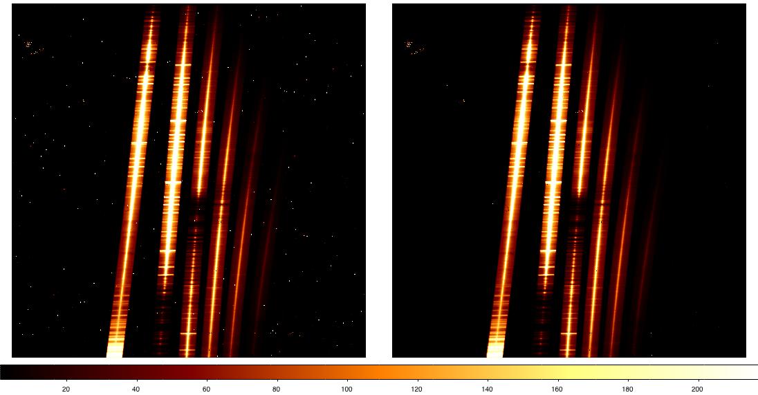
At this stage the sky emission should have subtracted out and the spectral orders correctly cut (as discussed above). The figure below shows how a raw and reduced galaxy (upper panels) and standard star file appear at this point (displayed using the display and nxdisplay commands)
We now have a couple of sky-subtracted, flatfielded galaxy and standard star spectra at each nod position. These individual spectra need to be combined. For the galaxy, we have two on-object spectra at the same nod position, and two blank sky spectra. We will use nscombine to simply average the two sky-subtracted, on-source files. For the telluric standard we will use nscombine to shift and average the nod beams. Because we have already cleaned the files of radiation events, we won't attempt any pixel rejection in nscombine or nsstack. If that had not been done, we could investigate using the "rejtype" and associated parameters to reject affected pixels.
ecl> imdelete rclnN20110516S0155_comb verify- >& dev$null
ecl> nscombine rclnN20110516S0155,rclnN20110516S0159 rejtype=none masktype=none
ecl> imdelete rclnN20110516S0186_comb verify- >& dev$null
ecl> nscombine rcln@telluric.lis rejtype=none masktype=none
The overall appearance of the galaxy data changes little during this procedure, but each order of the standard star (or a science target that didn't nod off the slit) should now have a single, central positive spectrum and two flanking negative spectra.

S-distortion correction and wavelength calibration
As the spectral orders are tilted and curved, the next step in the reduction is to rectify them. We also measure and apply the wavelength calibration at this stage.
The nssdist task is used to measure the spectral distortion, which it does by tracing the pinhole flatfield spectra across the array (a standard star stepped along the slit could also be used). The user needs to use the coordlist parameter to specify the file containing the pinhole coordinates. These files reside in the gnirs$data directory; in this case the user should pick the pinholes-short-dense-north.lis file, signifying the short (0.15"/pix") camera and GNIRS at Gemini North.
ecl> nssdist rnN20110516S0379 coordlist=gnirs$data/pinholes-short-dense-north.lis
function="legendre" order=5  minsep=5 thresh=1000 nlost=0 fl_inter+
When run interactively, nssdist presents a cross-section of the pinholes for each order. Use the "m" key to mark each pinhole (followed by <Enter>), ignoring any faint ones that may be vignetted by the decker (the mechanism that defines the length of the slits). The first two of the three numbers that appear in the irafterm window are the pixel position of the selected peak. The third number in the parentheses is the expected peak position from the file given by the coordlist parameter. The actual and expected numbers don't have to match exactly, but the difference between each measured peak and the expected peak given by the configuration file should be approximately the same in each order. Type "q" when finished to move to the next order. The task will give warnings about losing the trace in the higher orders; this is simply because there is little signal at the short wavelength ends of these orders.
We now run nswavelength on the arc(s) to establish the pixel-wavelength relation. Only one arc spectrum is required, but it is also possible to combine several arcs first to improve the S/N. In this user's experience nswavelength works reliably on arcs taken in this configuration. However it is a good idea to run the task interactively, at least initially, to check the results:
ecl> imdelete arc_comb verify- >& dev$null
ecl> nscombine rn@arcs.lis output="arc_comb"
ecl> imdelete warc_comb verify- >& dev$null
ecl> nswavelength arc_comb coordlist="gnirs$data/lowresargon.dat" fl_median+
threshold=300. nlost=10 fwidth=5. fl_inter+
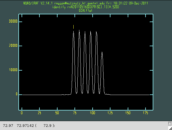
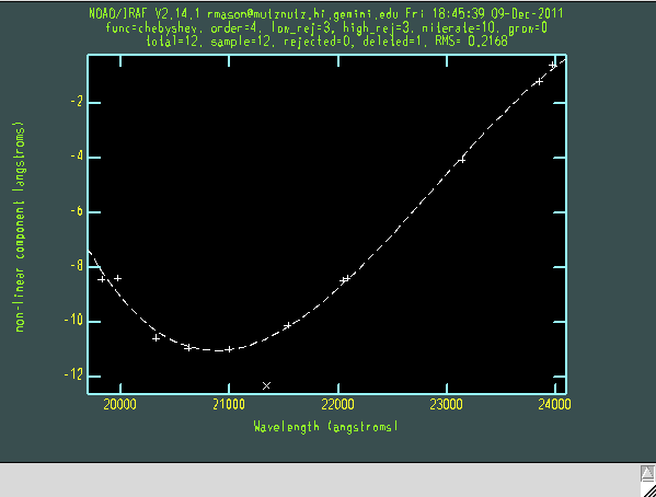
After applying an approximate wavelength solution based on information in the file headers and the gnirs$data/nsappwave.fits file, nswavelength asks the user whether they want examine line identifications interactively. Answering "yes" brings up the plot shown below. Hitting "f" shows the fit to the arc lines and allows the user to exclude lines by pressing "d" on any of the points. The "q" key returns to the initial plot (use "?" to see all keystroke options). Using "m" to mark a line will bring up its pixel position, fitted wavelength and the wavelength expected from the line list, information that can serve as a possible extra check of whether the line identification and fitting if working well. Arc line plots are available on the GNIRS (at R~5000) and UKIRT (at lower resolution) web pages and can serve as a useful sanity check at this stage. If the line wavelengths are acceptable, hit "q" to quit.
Nswavelength determines a 2D wavelength solution by stepping along the spatial axis and fitting the arc lines, creating a 2D map of the wavelengths along the whole slit. When nswavelength calls the reidentify task to identify the arc lines up and down the slit and asks "Fit dispersion function interactively?", it should not be necessary to examine the lines (answer "NO"). This process is repeated for each of the 6 orders.
The above call to nswavelength uses fl_median+. This is appropriate for data in which the arc lines are horizontal. GNIRS' detector is slightly tilted, so the arc lines are not exactly horizontal. Using fl_median+ appears to give acceptable results nonetheless, but users interested in precise wavelength calibration may be interested in setting fl_median- and supplying a pinhole file via the sdist parameter, in which case nswavelength calls nssdist and rectifies the arc lines. See the nswavelength help for more information.

To actually apply the distortion correction and wavelength calibration to the data, it is necessary to run the galaxy and standard star files through nsfitcoords and nstransform. Nsfitcoords creates database files containing information that nstransform applies to the data; nsfitcoords does not actually alter the data itself. Normally, nsfitcoords must be run interactively:
ecl> imdelete frclnN20110516S0155_comb,frclnN20110516S0186_comb  verify- >& dev$null
ecl> nsfitcoords rclnN20110516S0155_comb lamptrans="warc_comb"
sdisttrans="rnN20110516S0379" fl_inter+ lxorder=1 lyorder=3 sxorder=4 syorder=4
ecl> nsfitcoords rclnN20110516S0186_comb lamptrans="warc_comb"
sdisttrans="rnN20110516S0379" fl_inter+ lxorder=1 lyorder=3 sxorder=4 syorder=4
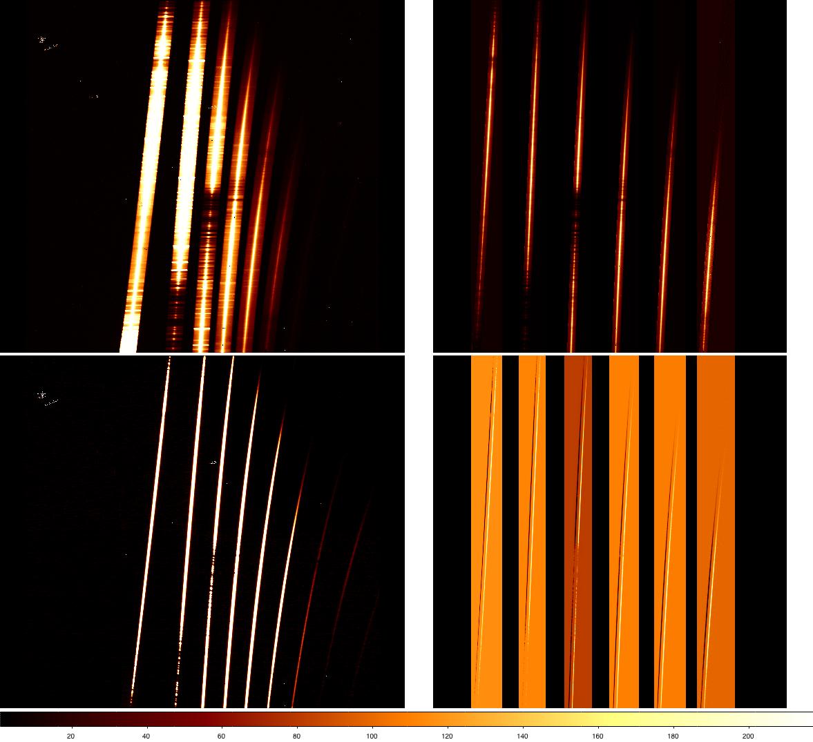
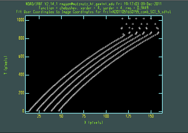
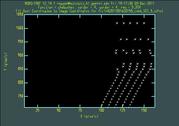
For each order, nsfitcoords presents arc lamp and pinhole plots. Probably the most useful sequence of keystrokes to use on the plots is "xxyyr". This brings up a plot of x pixel vs y pixel, and the title of the plot (containing "lamp" or "sdist") shows whether the wavelength or s-distortion solution is the one being checked. The lower orders are quite well-behaved, but it is usually necessary to delete points from the s-dist plots for the higher orders. For example, the figure below shows the initial s-dist plot, the plot shown after typing "xxyyr", and a close-up of points deleted from the fit (using the "d" and "y" keys), for order 5. It is important that the same s-distortion and wavelength solutions be applied to the science and standard star data. This means that any points that are deleted in one call to nsfitcoords should also be deleted in the other.

We now run nstransform on both data sets:
ecl> imdelete tfrclnN20110516S0155_comb,tfrclnN20110516S0186_comb verify- >& dev$null
ecl> nstransform frclnN20110516S0155_comb,frclnN20110516S0186_comb
By this stage in the reduction we have a single straightened, wavelength-calibrated file for the galaxy and the same for the telluric standard. After running nstransform on the data, the wavelength scale is inverted compared to the raw files. To check that the wavelength calibration is acceptable we could, for example, run nsfitcoords and nstransform on the arc itself, use nsextract or imcopy and splot to extract and plot a spectrum, and compare the line wavelengths against a reference spectrum such as those on the web pages mentioned above. As a rough check of the rectification of the spectra, we could use imexam's "j" command to fit Gaussians at various points and check that the fitted centre does not change appreciably along the spectrum.

Extracting spectra
The spectra are now ready to be extracted. The nsextract task has many options, and the most suitable ones will depend on the characteristics of the data set and the purpose(s) the spectra are to be used for. The spectra should be very close to vertical after the rectification performed above, so one possibility is to simply extract and sum a few columns. For bright objects like this galaxy and standard star, nsextract can automatically locate the peak of the spectrum and the task could be run non-interactively.
ecl> imdelete vtfrclnN20110516S0155_comb,vtfrclnN20110516S0186_comb verify- >& dev$null
ecl> nsextract tfrclnN20110516S0155_comb up=6 low=-6 ylevel=INDEF fl_apall-
fl_project+ background=none outprefix=v
ecl> nsextract tfrclnN20110516S0186_comb up=6 low=-6 ylevel=INDEF fl_apall-
fl_project+ background=none outprefix=v
We could also extract the data using apall. For XD spectra extracted using apall within nsextract, various default extraction parameters (upper and lower aperture limits, etc.) are specified order-by-order in the gnirs$data/apertures.fits table. If these values do not suit the user's needs, several options are available:
- Setting fl_usetabap- on the command line causes the aperture values in the aperture table to be ignored in favour of the user's upper and lower aperture limits, as in the example below.
- Many parameters can be changed interactively while running nsextract
- The user can create a copy of the gnirs$data/apertures.fits file and edit it to contain values optimised for their particular data set. This table is passed to nsextract using the "aptable" parameter
See the nsextract help for more information on these options.
Using apall's tracing functionality on the standard star data allows us to verify that the spectra were indeed straightened correctly in previous steps, and to correct for any small deviations if desired. We can then extract the galaxy spectra using the trace measured for the standard star. Because the galaxy fills the slit, we will disable background subtraction when extracting its spectra.
ecl> imdelete xtfrclnN20110516S0186_comb verify- >& dev$null
ecl> nsextract tfrclnN20110516S0186_comb fl_project- fl_apall+ fl_trace+ fl_inter+
ecl> imdelete xtfrclnN20110516S0155_comb verify- >& dev$null
ecl> nsextract tfrclnN20110516S0155_comb up=6 low=-6 fl_usetabap- fl_project- fl_apall+
background="none" fl_addvar- fl_trace- trace=tfrclnN20110516S0186_comb fl_inter+
When extracting the galaxy in this way, we say "no" when asked if we want to resize the aperture and then use the "s" key to shift the aperture so that it is properly centred on the emission peak.
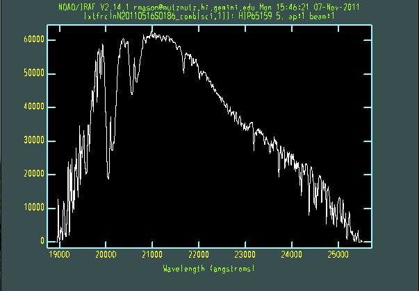
The extracted galaxy and standard star spectra are shown below.

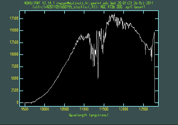

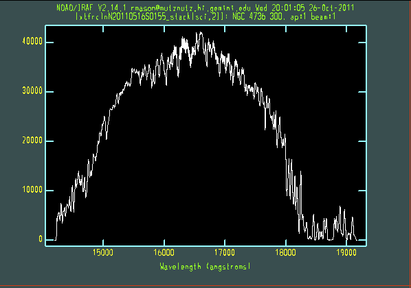


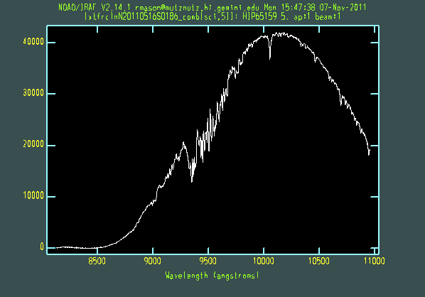

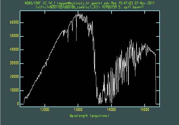

Telluric line cancellation
Several options are available at this stage. The nstelluric task can be used to shift and scale the standard star for (in theory) the best telluric line cancellation. Use of nstelluric is somewhat involved; the "msabsflux" section of this web page gives some hints that are also applicable to nstelluric. Alternatively, the native IRAF telluric and calibrate tasks can be run on each extension to shift, scale and ratio the spectra and apply a spectrophotometric calibration to the data. Users familiar with the Starlink software could instead use Figaro's scross, ishift and irflux tasks on each galaxy extension. Users familiar with Spextool and/or IDL may be interested in using the xtellcor package.
For this example, we will simply divide the galaxy by the standard star and then multiply by a blackbody of appropriate temperature. (To improve the telluric cancellation, the fxcor and imshift tasks in the noao.rv and images.imgeom packages could be used on each extension to cross-correlate and shift the spectra before dividing.) The blackbody spectra will need to span the same range of wavelengths as the real data. This can be determined using the hselect command to show the starting wavelength and wavelength increment, or by writing the spectra into text files and examining the start and end wavelengths in a text editor:
hselect vtfrclnN20110516S0155_comb[sci,1] field=$I,CRVAL1,CD1_1 expr="yes"
#vtfrclnN20110516S0155_comb[sci,1]       18938.51171875  6.43956995010377
onedspec
delete temp*
wspectext vtfrclnN20110516S0155_comb[sci,1] temp1 header-
#Starting wavelength = 18939 Angstroms, ending wavelength = 25513 Angstroms
We also need to know the spectral type and temperature of the standard star. The spectral type can be found using SIMBAD, for example, and this web page is a useful source of stellar temperatures. This particular standard star, HIP 65159, is of spectral type F8V with a temperature of approximately 6100 K. Depending on the spectral type of the standard star, it may be desirable to model out lines originating in the standard star itself during this process.
So, to conclude the reduction, we perform something like this set of steps on each extension of the extracted galaxy file:
delete N4736_3.fits verify- >& dev$null
imarith vtfrclnN20110516S0155_comb[sci,1]  / vtfrclnN20110516S0186_comb[SCI,1] result=N4736_3
imdel order3_6100K verify- >& dev$null
mk1dspec order3_6100K ncols=1022 wstart=18939  wend=25513 temperature=6100
imdel N4736_3_bb verify- >& dev$null
imarith N4736_3 * order3_6100K result=N4736_3_bb
delete bb_orders.txt verify- >& dev$null
files N4736_*bb.fits > bb_orders.txt
delete txt*bb.fits verify- >& dev$null
wspectext @bb_orders.txt txt@bb_orders.txt header=no
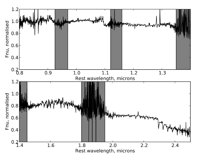
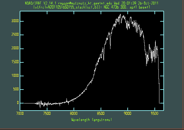
The resulting galaxy spectrum is shown below with the orders merged together and the flux normalised around 1 micron. Given the narrow slit and non-photometric conditions under which these observations were obtained, no flux calibration was attempted during this reduction. This could be accomplished by scaling the spectrum to existing photometry of the galaxy, if data in a similar aperture is available. The grey bars show some regions of strong atmospheric absorption (see e.g. these sky transmission spectra). Some of the "noise" and features in the spectrum, especially in orders 3 and 4, are probably in fact real, distinct absorption features in cool stars in the target galaxy itself.