
| You are in: Instruments > MIR > Example Q Band Reduction |  |
 |
Example Michelle Q Band Reduction |
This is an example of using the msreduce script to reduce a Q-band spectrum. In this instance one has an observation of an asteroid and an observation of a standard star both at Q-band in the lowres20 mode of Michelle. These were in fact both calibration objects used for a Michelle queue programme, but here we will treat the asteroid as if it were the science target. The raw data file for the asteroid observation is N20060621S0194.fits while the raw data file for the standard star observation is N20060621S0210.fits. The star is HD175775, one of the brighter Cohen standards. It is bright enough to be used as a standard for Q-band spectroscopy in good conditions; the Qa in-band flux density is 5.794 Jy. The asteroid is 261 Prymno, which has an estimated radius of 25.5 km and was at a distance of 1.35 A.U. at the time of observation. This gives an estimated brightness of 12.2 Jy in the Qa filter, so it is expected to be twice as strong as the star. This is not particularly bright for an asteroid calibrator used with Michelle, generally a larger asteroid would be preferred.
The first step is run the nsheaders to set the instrument to Michelle.
cl> nsheaders michelle
------------------------------------------------------------------------------
NSHEADERS -- Mon Nov 27 12:47:12 HST 2006

setting header keywords
setting nscut.section
setting nsreduce.section
resetting nswavelength.dispaxis
setting nswavelength.coordlist, nswavelength.threshold, and
   nswavelength.fl_median
setting the default logfile
Then one has to set the parameters for nsreduce as follows: (except that the rawpath value need not be as indicated here)
cl> lpar msreduce
       inspec = "N20060621S0194" Name of source spectrum raw data file(s)
     (outtype = "fnu")          Type of output spectrum: fnu|flambda|lambda*flambda
     (rawpath = "rawdata")      Path for raw images
        (line = 160)            Line to use to identify the aperture
      (fl_std = yes)            Extract both source and standard spectra, do telluric correction
         (std = "N20060621S0210") Name of standard spectrum raw data file(s)
     (stdname = "HD175775")     Name of standard star
    (fl_bbody = no)             Use blackbody option rather than spectrophotometry
       (bbody = 10000.)         Temperature of calibrator for black-body fit
     (fl_flat = no)             Apply flat/bias to the raw data file(s) before processing
        (flat = "")             Input flat-field image(s) (raw data file(s))
        (bias = "")             Input bias image(s) (raw data file(s))
  (fl_extract = yes)            Run nsextract interactively
 (fl_telluric = yes)            Run msabsflux interactively
(fl_wavelengt = yes)            Run nswavelength interactively
(fl_transform = no)             Run nstransform interactively
  (fl_retrace = no)             Retrace spectrum, if appropriate
  (fl_process = yes)            Do initial processing with mprepare
    (fl_clear = yes)            Clear database sub-directory
 (fl_negative = no)             Extract from a negative spectrum (NOD mode)
 (fl_defringe = no)             Defringe the spectra (an intrinsicly interactive step)
   (fl_lowres = yes)            Low resolution spectrum [msdefringe]
        (fmin = 18)             Start of filtering region (pixels) [msdefringe]
        (fmax = 32)             End of filtering region (pixels) [msdefringe]
 (fl_dfinterp = yes)            Interpolate across masked region [msdefringe]
  (fl_zerocut = no)             Mask out negative points [msdefringe]
(fl_reextract = no)             Just re-extract the spectra
    (linelist = "gnirs$data/sky.dat") Line list file name
     (logfile = "example.log")  Log file name
     (verbose = yes)            verbose logging?
      (status = 0)              Exit error status: (0=good, >0=bad)
    (scanfile = "")             Internal use only
        (mode = "ql")
Note that the parameters are set with the standard star name and raw data file name, the raw data file name for the object, a path to these two raw data files, and various of the flags are set. In this case there is no need to do de-fringing so fl_defringe is set to "no". Most of the other parameters have their default values.
Before starting the reduction it is useful to look at the raw data and see (a) what the atmospheric emission lines look like, so one can get a rough ID of the features, and (b) whether the spectrum needs to be defringed. This can be done from the raw data files if one wishes, as in
cl> display rawdata/N20060621S0194[1][*,*,3,1] zs- zr+ nsample=76800

cl> imexam

cl> display rawdata/N20060621S0194[1][*,*,1,1] zs- zr+ nsample=76800

cl> imexam
The first display command shows the raw data from one nod position, the first nod A position, for the object plus the sky. The way this looks in ds9 is as follows--
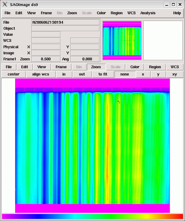
One sees the strong atmospheric lines, and the source is much too faint to be seen in the raw image. In imexam one then can do a line cut with the "l" cursor key to get a cut across the image--
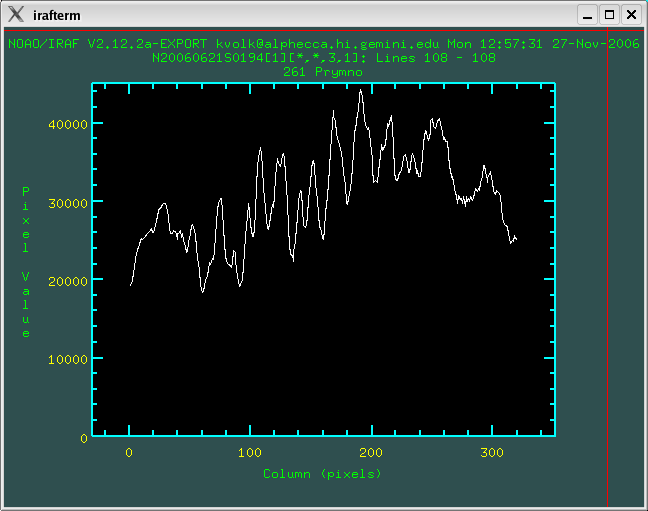
This figure has been made with the y range set from 0 to 45000 ADU to show the true line to continuum contrast in fairly dry conditions at Mauna Kea.
The next display command displays the difference spectral image from the same nod, wherein the object spectrum can be seen--
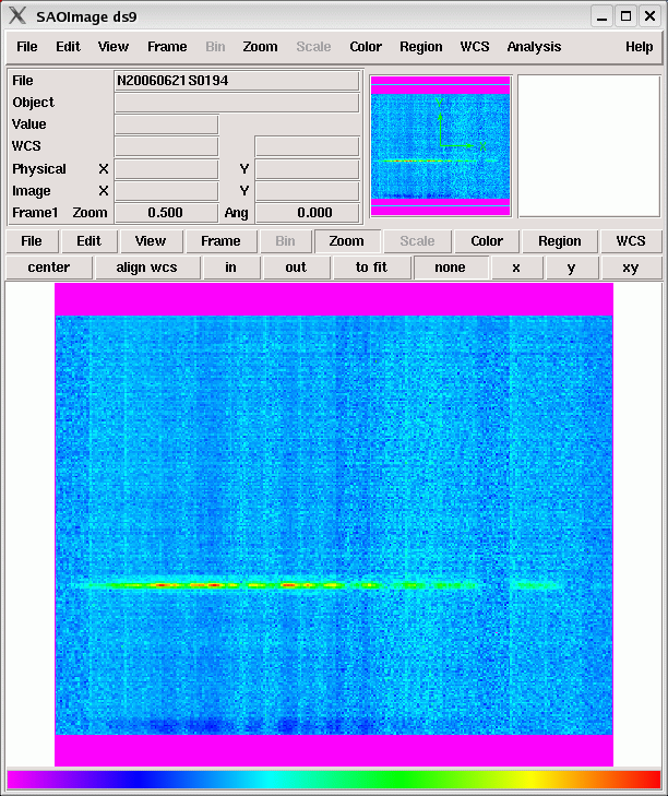
The raw spectrum is interrupted frequently by the atmospheric bands where the background is high and the atmospheric transmission is low. A line cut along the peak of the spectrum looks like this--
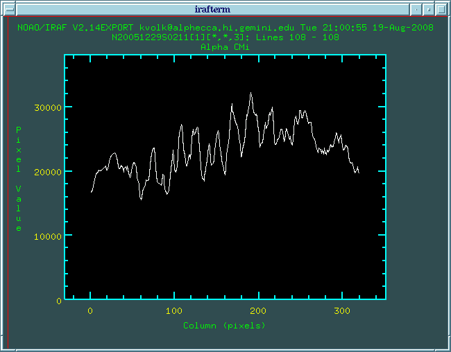
where one sees the atmospheric lines as absorption lines instead of emission lines. There is no fringing in this line cut, so de-fringing of the spectrum is not needed.
Of note is that the band at about 20 microns, near pixel 135, has split into two peaks at this resolution, and so it is not usable for the wavelength calibration.
The call to msreduce can either be done by editing the parameters to the values listed above or by the command
cl> msreduce N20060621S0194 std=N20060621S0210 stdname="HD175775"\
fl_defringe- rawpath="rawdata"
provided that the various flags were set properly using epar. In a script the form of the call would be
msreduce ("N20060621S0194",
outtype="fnu", rawpath="rawdata", line=160, fl_std=yes, std="N20060621S0210",
stdname="HD175775",fl_bbody=no, bbody=10000., fl_flat=no, flat="", bias="",
fl_extract=yes,fl_telluric=yes, fl_wavelengt=yes, fl_transform=yes, fl_retrace=no,
fl_process=yes, fl_clear=yes, fl_negative=no, fl_defringe=no, fl_lowres=yes,
fmin=18, fmax=32, fl_dfinterp=yes, fl_zerocut=no, fl_reextract=no,
linelist="gnirs$data/sky.dat", logfile="example.log", verbose=yes)
with the rawpath parameter having to be set to whatever directory is appropriate.
When one runs msreduce the task proceeds automatically until the wavelength calibration is to be done. The automatic line IDs are poor (see below) so one has to reset with the "i" key command and then find the lines. One marks the peaks with the "m" key and then enters the wavelength in Angstroms as listed below.
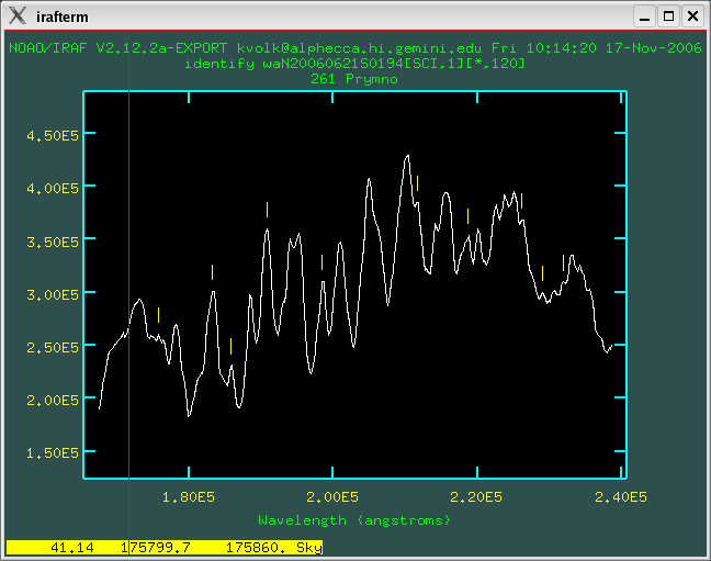
pixel 52     175860
pixel 75     182980
pixel 87     186480
pixel 98     190150
pixel 108    193100
pixel 141    203220
pixel 152    206530
pixel 169    211750
pixel 191    218550
pixel 215    225950
pixel 228    229410
pixel 234    231990
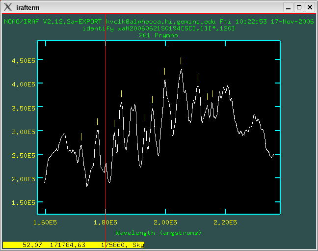
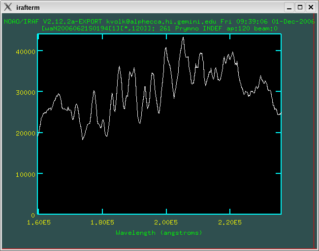
The wavelength calibration is good to within a few hundred Angstroms, or a few times 0.01 micron. If one needs higher precision than this one would have to work harder on the wavelength calibration aided by an atmospheric emission model at the proper resolution.
Once the initial wavelength calibration is carried out the nstransform routine finds the same features for different positions along the short axis of the image. For an extended source it might be useful to carry out this step interactively and so make sure that the IDs remain accurate over the range of slit positions where the source is seen. In this case it is not required to do this interactively.
The same process is then followed for the standard star, with the sky lines being at the same places as listed above, resulting in a wavelength calibrated sky spectrum for observation 210.
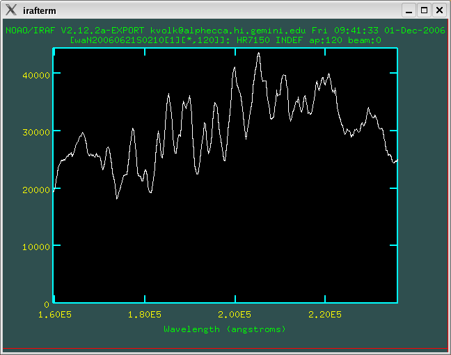
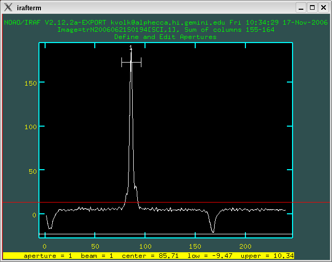
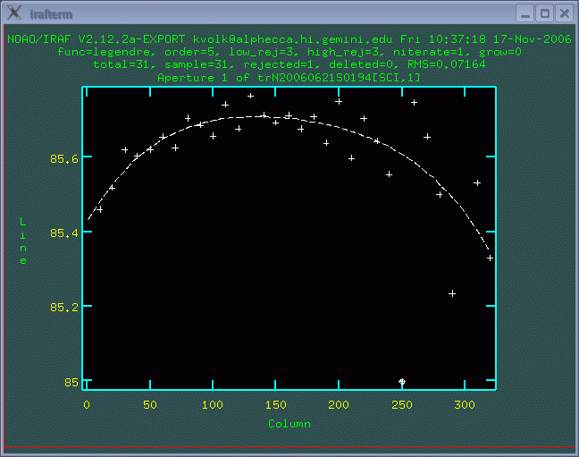
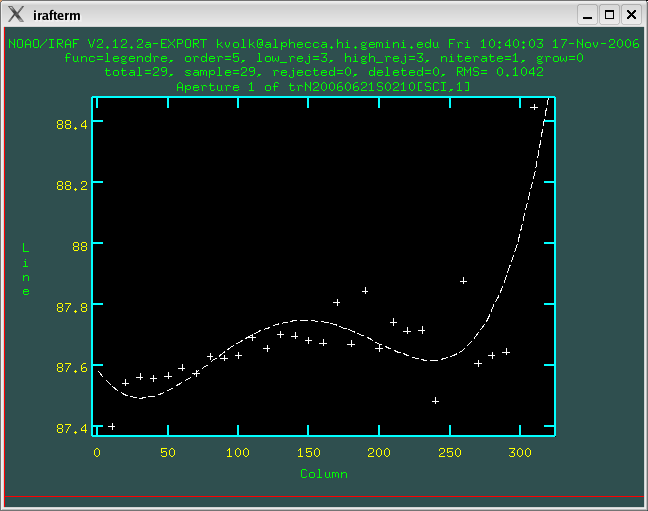
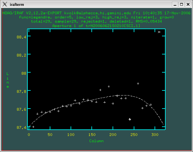
Next one has to choose the apertures for the object and for the standard, in this case these were chosen to get all the flux as these two objects are point sources for Gemini at these wavelengths (the asteroid had an estimated angular diameter of 0.052 ac-seconds at the time of the observation). When the tracing is done, one needs to exclude a few points where there is no signal due to the atmosphere being opaque; the spectral tilt is small. For the calibration star the original tracing should be revised, so one should exclude one point with the "d" sky command and then re-fit with the "f" sky command.

Now the script produces wavelength calibrated raw spectra for the asteroid and for the calibration star, still rather badly chopped up by the atmospheric transmission.
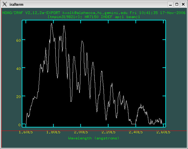
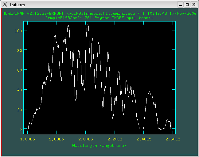
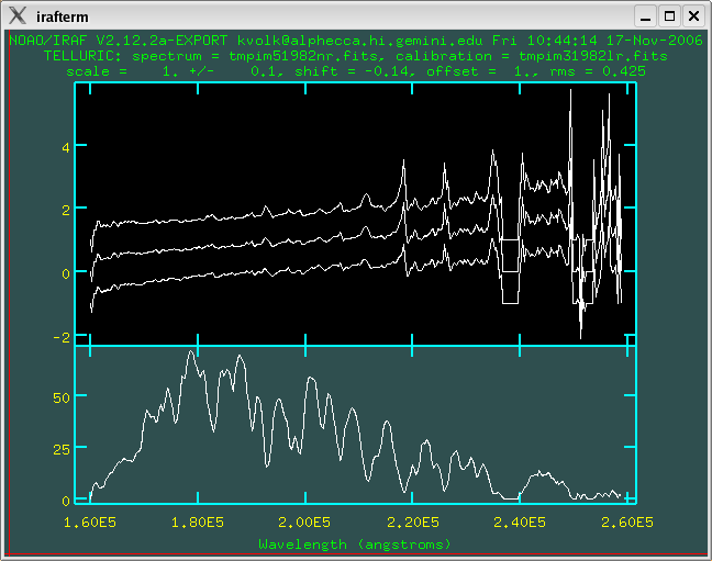
The method used here is to set dscale and offset to 0.0 with colon commands
:dscale 0.0
:offset 0.0
with one's cursor in the plot window. There is clear evidence of band mis-match as one sees the peaks at about 21.1, 21.8, 22.6, and 23.5 microns. These are all the minima of bands seen in the extracted spectra, so the character of the atmosphere changed between the two observations (they are separated by about 1.5 hours, as an observation of a science target was taken in the meantime). The goal was to find a shift that gives the smoothest output spectrum aside from these peaks, and to reduce the peaks themselves if possible. The best result obtained was for a shift of -0.5 pixels.
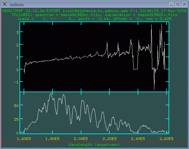
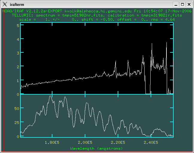
Even at the "best" shift the band centers show spikes, so the spectrum needs to be cleaned up to remove these points. Given the noise levels the spectrum is not too trustworthy beyond 24 microns. Interpolating across the "spikes" gives the spectrum shown below. We supplied the standard star name in the call to msreduce and set the fl_bbody flag to "no", so the resulting spectrum is calibrated in Jy.
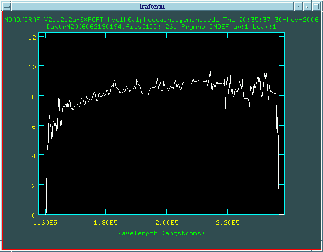
One now sees the calibrated spectrum for the asteroid.
The spectrum is rather noisy partly because the asteroid is not all
that bright and partly because of the difference in time between the
observations of the asteroid and standard star (which were observed
bracketing a science target). This result shows that the changes in
the atmosphere during the course of an observation can severely hamper
the results of ground-based Q-band spectroscopy. The water column
must have changed during the time period when these observations were
taken, resulting in the bands getting stronger. Thus for observations
of order 2 hours or more in total length it would be prudent to have
calibration observations both before and after the science observation
to see just how the atmosphere has changed. For Michelle spectroscopy
this is allowable as a baseline calibration for observations of
duration more than 2 hours. The situation is generally not as bad for
N-band spectroscopy where the atmospheric bands are weaker.
Last update 2006 December 04, K. Volk & R. Mason