Announcements
Components
GHOST provides high resolution optical spectroscopy at Gemini South, by using optical fibers connecting a cassegrain mounted integral field unit array to a bench spectrograph. The instrument can be divided into three main components, the bench spectrograph, the cassegrain unit, and the fibre array which each in turn can be subdivided into constitutent units. These charecterization of these components is given here. An overview of the instrument is given below.
Spectrograph components
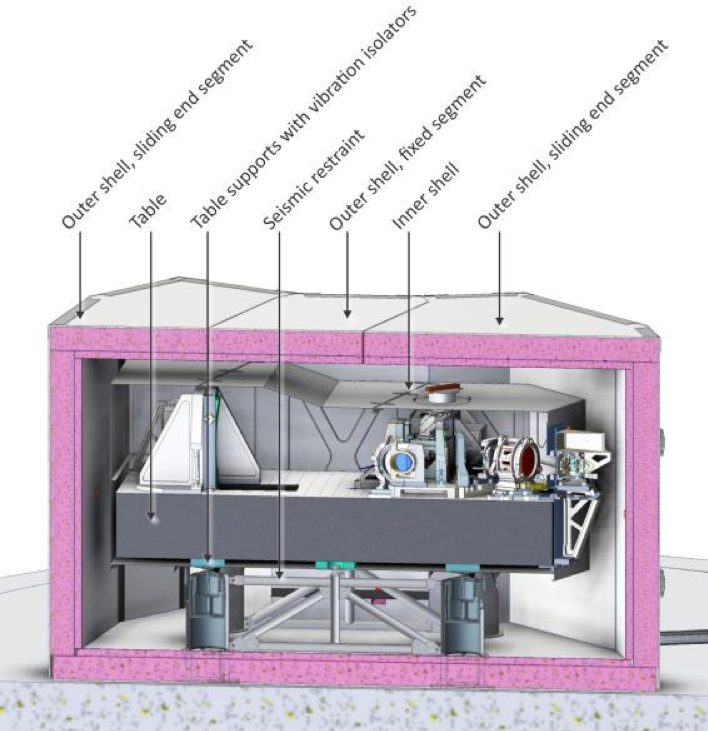
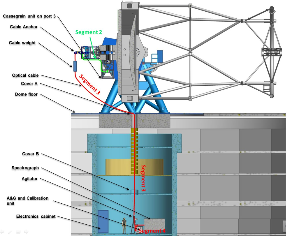
Light from the telescope is directed via the IFUs mounted on the cassegrain of Gemini South, and a 32m fibre cable to the spectrograph located in the pier lab of Gemini South, ensuring spectrograph stability. The bench spectrograph is a white-pupil cross-dispersed echelle, contained within a temperature-stabilized, pressure monitored enclosure.
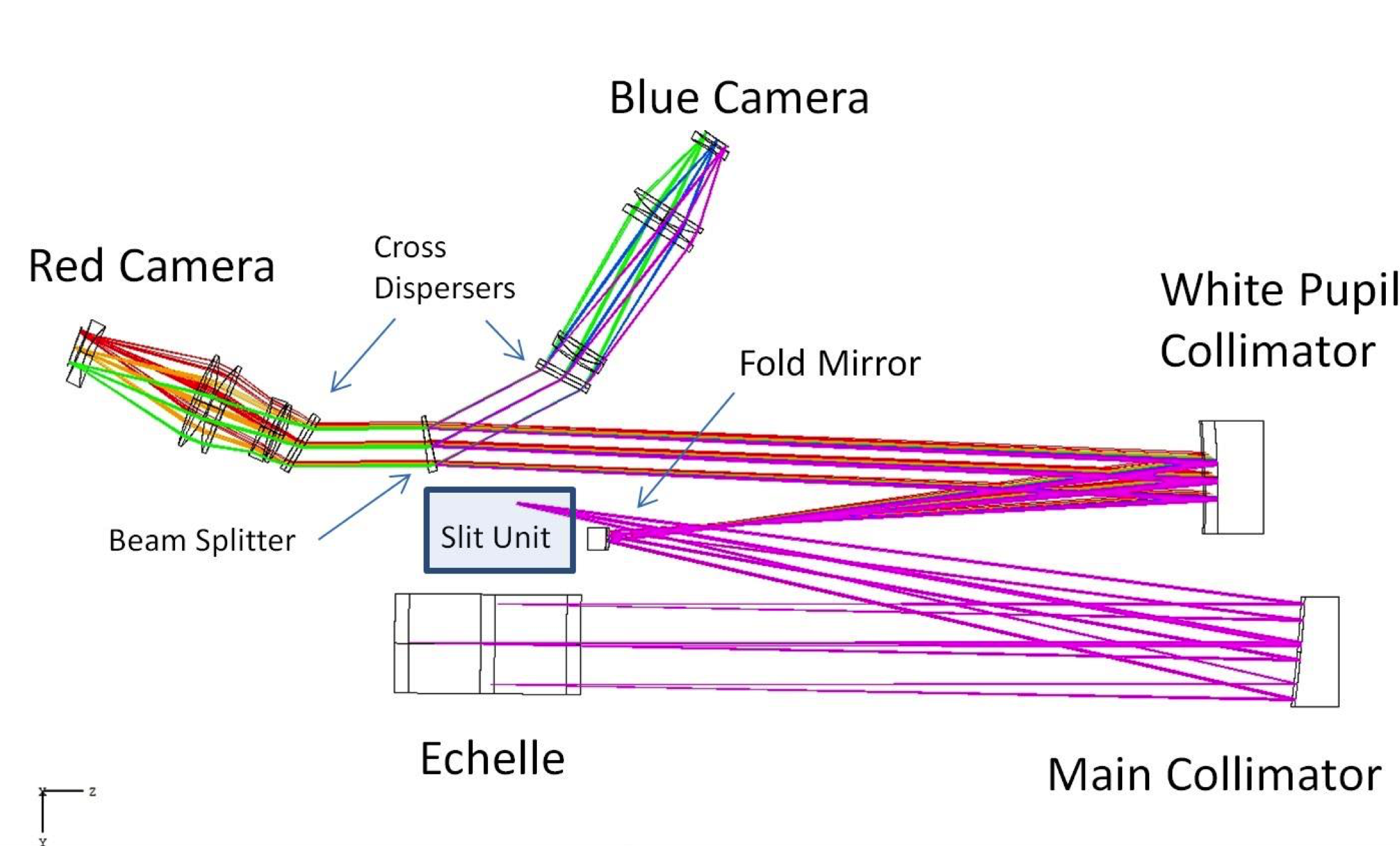
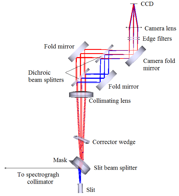
The echelle spectrograph has two arms separated by a dichroic at 530 nm. The light is relayed to the detectors using an asymmetric white pupil design with a Volume Phase Holographic Grating (VPHG) providing cross dispersion. Before this, approximately 1% of the light is captured by the slit unit, which contains linearly reformatted fibers, forming a psuedo-slit. This layout is illustrated in figure 1 below. Apart from the two camera shutters, there are no moving parts except for the slit mask. The temperature within the bench is controlled to within 5° of the nominal operating temperatures.
Detector Properties
Light from the two arms lands on two non-identical detectors, each having four amplifiers. Below we give the basic properties of the detectors, their read modes, and readout times in Table 1, 2, and 3. Flat fields are stable in both detectors over time, and you can safely use flats during the day for most science cases.
| Table 1: Summary of detector properties | |||||
|---|---|---|---|---|---|
| - | Blue | Red | |||
| Array | e2vCCD231-84 | e2vCCD231-c6 | |||
| Format | 4096x4112 | 6144x6160 | |||
| Overscan | 64 (H) | 64 (H) | |||
| Pixel size | 15µm | 15µm | |||
| Response | 347-542 nm | 520-1060 nm | |||
| Orders | 98 to 64 | 65 to 33 | |||
| Read rate | 10,5,2 µs pix-1 (2,4, and 8 ports) | 10,5,2 µs pix-1 (2,4, and 8 ports) | |||
| Dark | ≤ 1.0 e- pix-1 hr-1 | ≤ 0.9 e- pix-1 hr-1 | |||
| Amplifiers | Four | Four | |||
| Full Well Depth | 350000 e- | 350000 e- | |||
| Saturation | 65000 ADU | 65000 ADU | |||
| Gain | ≤ 0.61 e- DN-1 | ≤ 0.57 e- DN-1 | |||
| Bias | ~ 200 ADU | ~ 400 ADU | |||
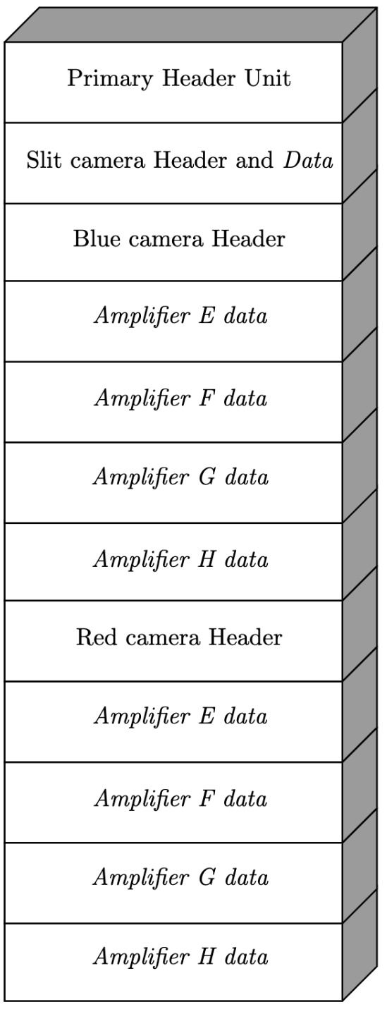
The final MEF format is given above. The multi-extension FITS format for a single science image in both red, and blue cameras, and the slit viewing camera. The format is of the delivered data.
| Table 2: Summary of read modes | ||||||
|---|---|---|---|---|---|---|
| Read modes in blue | ||||||
| Read Mode | Read Noise* (e-) |
Gain* (e-/DN) |
Comments | |||
| SLOW | 2.1 | 0.5 | Recommended read mode in blue | |||
| MEDIUM | 2.5 | 0.57 | ||||
| FAST | 4.6 | 0.73 | ||||
| Read modes in red | ||||||
| Read Mode | Read Noise* (e-) |
Gain* (e-/DN) |
Comments | |||
| SLOW | 2.2 | 0.51 | ||||
| MEDIUM | 2.55 | 0.55 | Recommended read mode in red | |||
| FAST | 4.4 | 0.7 | ||||
*The read noise and gain are the mean values over all amplifiers.
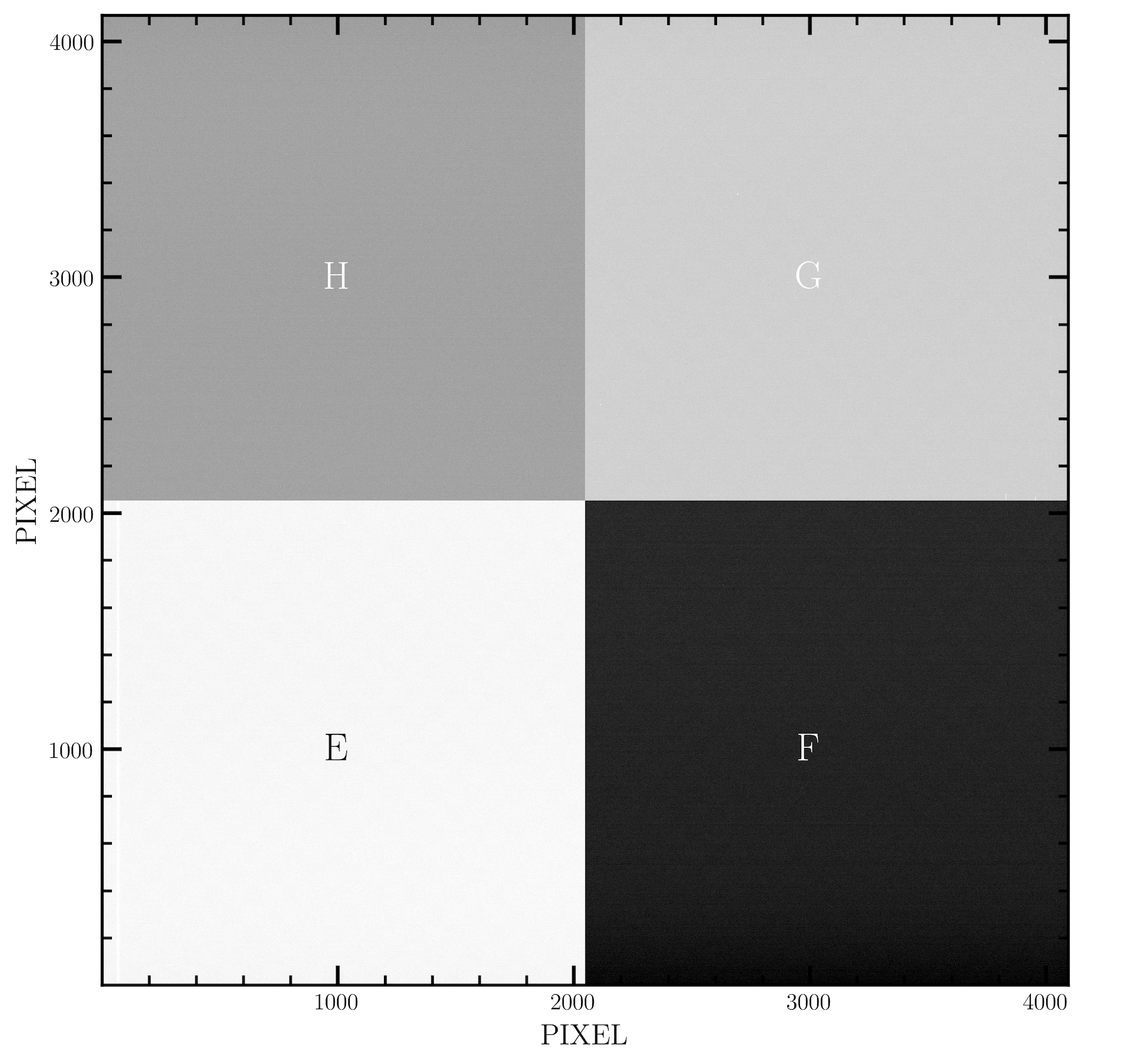
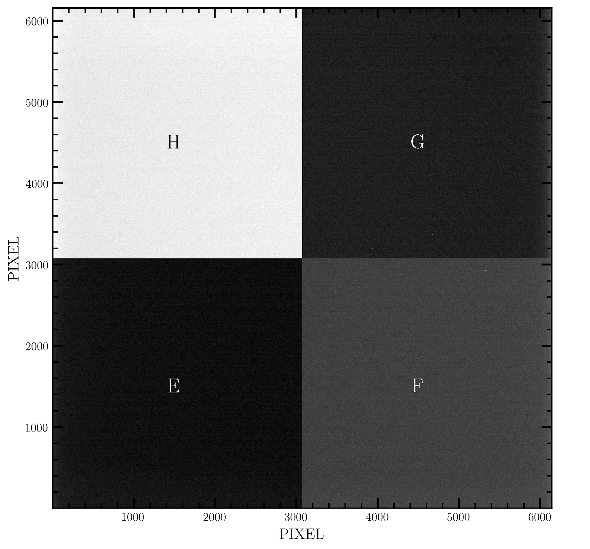
The final image with each amplifiers labelled is shown below
The readout times for both detectors are given below in each binning and read mode.
| Table 3: Readout overheads | |||||
|---|---|---|---|---|---|
| - | Spectral binning | Spatial binning | Red read time (s) | Blue read time (s) | |
| SLOW | 1 | 1 | 97.4 | 45.6 | |
| SLOW | 1 | 2 | 49.6 | 24.8 | |
| SLOW | 1 | 4 | 25.7 | 14.4 | |
| SLOW | 1 | 8 | 13.8 | 9.1 | |
| SLOW | 2 | 2 | 27.5 | 15.4 | |
| SLOW | 2 | 4 | 14.7 | 9.8 | |
| SLOW | 2 | 8 | 8.4 | 7.0 | |
| SLOW | 4 | 4 | 9.5 | 7.9 | |
| MEDIUM | 1 | 1 | 50.1 | 24.6 | |
| MEDIUM | 1 | 2 | 26.1 | 14.3 | |
| MEDIUM | 1 | 4 | 13.9 | 9.1 | |
| MEDIUM | 1 | 8 | 7.9 | 6.5 | |
| MEDIUM | 2 | 2 | 15.7 | 10.1 | |
| MEDIUM | 2 | 4 | 8.8 | 7.2 | |
| MEDIUM | 2 | 8 | 5.4 | 5.6 | |
| MEDIUM | 4 | 4 | 6.5 | 6.5 | |
| FAST | 1 | 1 | 21.7 | 12.0 | |
| FAST | 1 | 2 | 11.7 | 7.9 | |
| FAST | 1 | 4 | 6.8 | 5.9 | |
| FAST | 1 | 8 | 4.3 | 4.9 | |
| FAST | 2 | 2 | 8.6 | 6.9 | |
| FAST | 2 | 4 | 5.2 | 5.6 | |
| FAST | 2 | 8 | 3.6 | 4.9 | |
| FAST | 4 | 4 | 4.7 | 5.8 | |
Slit unit
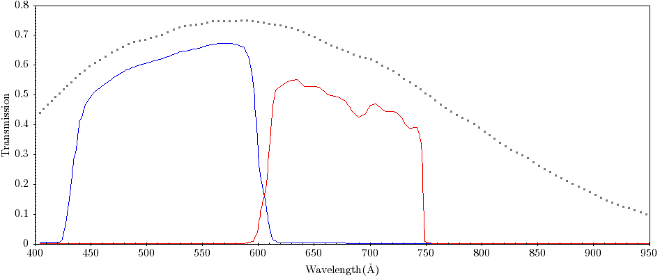
Before light enters the spectrograph, it is horizontally displaced from the IFUs, effectively slicing the image. This slit unit absorbs 1% of all light entering the bench, and is shown in the figure below. The slit is dispersed through custom filters, one allowing light from 420-600nm (the blue slit), and the other from 600-760nm (the red slit.) The final slit profile is not a Gaussian, but follows a Box shape, and can be approximated using a factor of 1.18. Below follow a quick summary of the slit unit and its detector. Properties of the slit unit are given in Table 4.
| Table 4: Slit unit | |
| Detector Array | Sony ICX674 |
| Detector format | 300 x 240; 4.54 micron pixels |
| Spectral Response | 400-1000 nm |
| Detector Dark Current* | 0.02 e-/s/pix |
| Saturation | 16,000 ADU |
| Slit tilt | 9° |
| Slit filters | 420-600nm (blue) 600-700nm (red) |
| Quantum efficiency | 40% at 400nm 75% at 600nm |
| Residual image retention | Minimal impact on science |
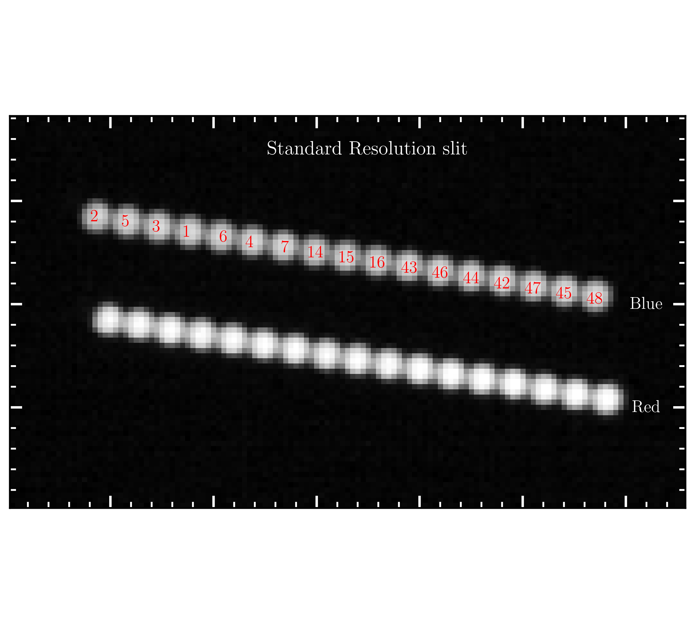
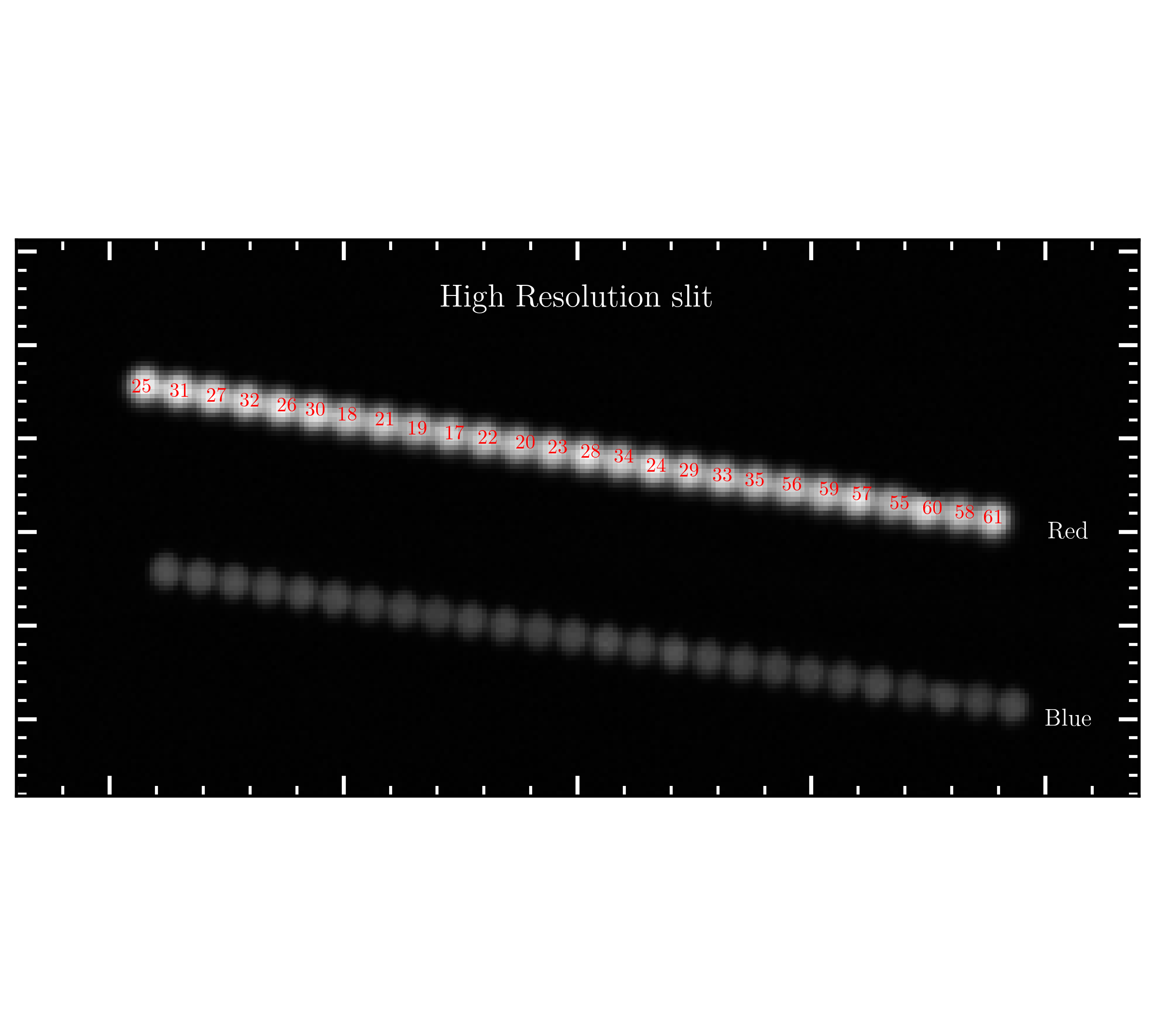
The slit images are always obtained in 2x2 binning; with the readout time less than 0.1s. The minimum exposure time is 0.1s. An example flat image of the slit viewing camera is shown below for illustration. The full width half maximum is measured using the reprojected images of the psuedo-slit, and is recorded in each slit viewing image header following the keywords INNBFWHM, or INNRFWHM, where NN refers to either the IFU1 or IFU2 High or Standard resolution, blue and red slit respecitvely.
Echelle grating and dispersers
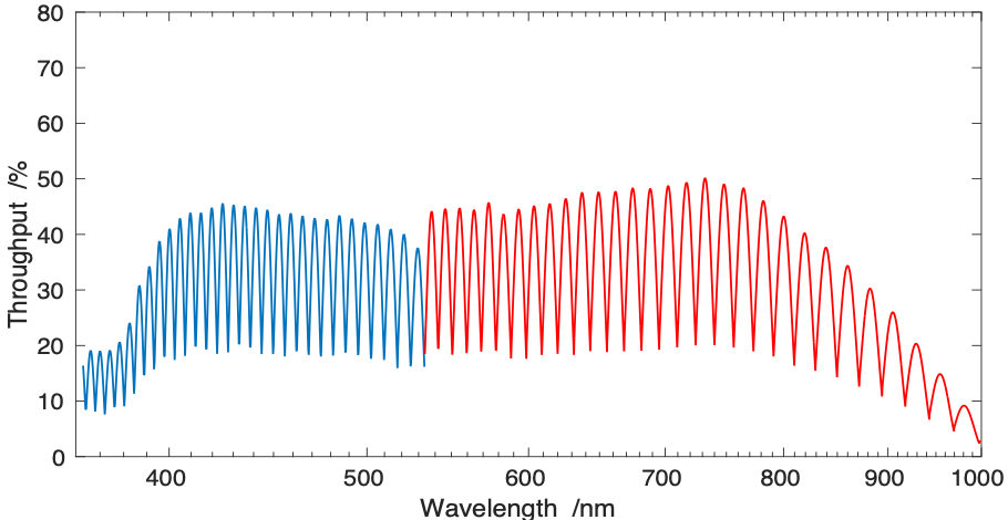
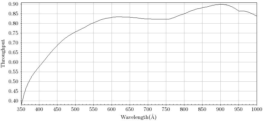
The echelle was procured from Richardson Grating Labs. The grating 424E R-2.14 has a line frequency of 52.67 grooves/mm, with blaze angle of 65°. The exact master used was MR234. The grating has maximum diffraction efficiencies of 80% at the centre of each order, allowing for better throughput at the order centers. The throughput of the echelle is given below, with Table 5 providing a summary of the orders.
Before light arrives on the science cameras, a VPHG cross-disperser is used. For the blue, this has 1050 lines/mm, and fringe of 35°. The red has 500 lines/mm, with a 31° fringe. Both dispersers are made from fused silica, in a non-Littrow configuration.
| Table 5: Summary of echelle grating | |||||
|---|---|---|---|---|---|
| Order | Wavelength (nm) | Free spectral range (nm) | CCD (nm) | Ratio | |
| 95.0 | 362.2 | 4.27 | 8.22 | 1.92 | |
| 94.0 | 366.1 | 4.36 | 8.29 | 1.90 | |
| 93.0 | 370.0 | 4.46 | 8.36 | 1.87 | |
| 92.0 | 374.1 | 4.55 | 8.44 | 1.85 | |
| 91.0 | 378.2 | 4.65 | 8.52 | 1.83 | |
| 90.0 | 382.4 | 4.76 | 8.6 | 1.80 | |
| 89.0 | 386.7 | 4.87 | 8.68 | 1.78 | |
| 88.0 | 391.1 | 4.98 | 8.77 | 1.76 | |
| 87.0 | 395.6 | 5.09 | 8.85 | 1.73 | |
| 86.0 | 400.2 | 5.21 | 8.94 | 1.71 | |
| 85.0 | 404.9 | 5.34 | 9.03 | 1.69 | |
| 84.0 | 409.7 | 5.46 | 9.13 | 1.67 | |
| 83.0 | 414.6 | 5.59 | 9.22 | 1.64 | |
| 82.0 | 419.7 | 5.73 | 9.32 | 1.62 | |
| 81.0 | 424.9 | 5.88 | 9.43 | 1.60 | |
| 80.0 | 430.2 | 6.02 | 9.53 | 1.58 | |
| 79.0 | 435.6 | 6.18 | 9.64 | 1.55 | |
| 78.0 | 441.2 | 6.34 | 9.75 | 1.53 | |
| 77.0 | 446.9 | 6.5 | 9.86 | 1.51 | |
| 76.0 | 452.8 | 6.67 | 9.98 | 1.49 | |
| 75.0 | 458.8 | 6.85 | 10.1 | 1.47 | |
| 74.0 | 465.0 | 7.04 | 10.23 | 1.45 | |
| 73.0 | 471.4 | 7.23 | 10.36 | 1.43 | |
| 72.0 | 478.0 | 7.44 | 10.5 | 1.41 | |
| 71.0 | 484.7 | 7.65 | 10.64 | 1.39 | |
| 70.0 | 491.6 | 7.87 | 10.78 | 1.36 | |
| 69.0 | 498.7 | 8.09 | 10.93 | 1.35 | |
| 68.0 | 506.1 | 8.34 | 11.08 | 1.32 | |
| 67.0 | 513.6 | 8.59 | 11.24 | 1.30 | |
| 66.0 | 521.4 | 8.85 | 11.4 | 1.28 | |
| 65.0 | 529.4 | 9.12 | 11.58 | 1.26 | |
| 64.0 | 537.7 | 9.41 | 11.76 | 1.24 | |
| 63.0 | 546.2 | 9.71 | 18.42 | 1.89 | |
| 62.0 | 555.1 | 10.03 | 18.71 | 1.86 | |
| 61.0 | 564.2 | 10.36 | 19.02 | 1.83 | |
| 60.0 | 573.6 | 10.71 | 19.33 | 1.80 | |
| 59.0 | 583.3 | 11.07 | 19.65 | 1.77 | |
| 58.0 | 593.3 | 11.46 | 19.98 | 1.74 | |
| 57.0 | 603.7 | 11.86 | 20.33 | 1.71 | |
| 56.0 | 614.5 | 12.29 | 20.69 | 1.68 | |
| 55.0 | 625.7 | 12.74 | 21.06 | 1.65 | |
| 54.0 | 637.3 | 13.22 | 21.45 | 1.62 | |
| 53.0 | 649.3 | 13.72 | 21.85 | 1.59 | |
| 52.0 | 661.8 | 14.25 | 22.27 | 1.56 | |
| 51.0 | 674.8 | 14.82 | 22.7 | 1.53 | |
| 50.0 | 688.3 | 15.42 | 23.16 | 1.50 | |
| 49.0 | 702.3 | 16.05 | 23.63 | 1.47 | |
| 48.0 | 717.0 | 16.73 | 24.12 | 1.44 | |
| 47.0 | 732.2 | 17.45 | 24.63 | 1.41 | |
| 46.0 | 748.1 | 18.21 | 25.16 | 1.38 | |
| 45.0 | 764.7 | 19.03 | 25.73 | 1.35 | |
| 44.0 | 782.1 | 19.91 | 26.31 | 1.32 | |
| 43.0 | 800.3 | 20.85 | 26.92 | 1.29 | |
| 42.0 | 819.4 | 21.85 | 27.57 | 1.26 | |
| 41.0 | 839.4 | 22.93 | 28.24 | 1.23 | |
| 40.0 | 860.3 | 24.09 | 28.95 | 1.20 | |
| 39.0 | 882.4 | 25.34 | 29.7 | 1.17 | |
| 38.0 | 905.6 | 26.69 | 30.48 | 1.14 | |
| 37.0 | 930.1 | 28.15 | 31.31 | 1.11 | |
| 36.0 | 955.9 | 29.74 | 32.18 | 1.08 | |
| 35.0 | 983.2 | 31.46 | 33.11 | 1.05 | |
| 34.0 | 1012.2 | 33.34 | 34.09 | 1.02 | |
Internal calibration source
The fibres split the image in the focal plane, as image is injected into 7/19 microlenses separately, which is then vertically sliced onto the spectrograph. The resulting slit profiles are dependent on the injection conditions, resulting in poor radial scrambling. The slit image, while simultaneously imaging the slit, also accounts for the slightly different and seeing-dependent widths of the fiber profiles on the slit. In addition, an internal calibration source is also provided to obtain precise absolute calibration.
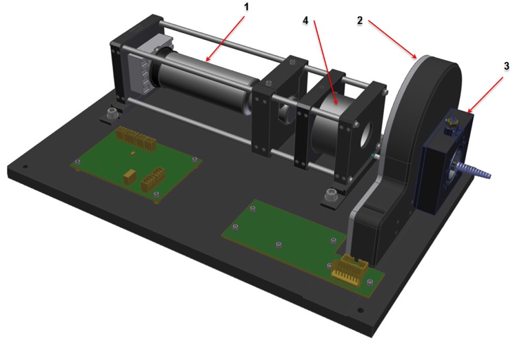
For this, the slit unit contains an internal ThXe lamp that can be turned on automatically during high-resolution spectral observations. The arc is translated to an additional microlens in the slit unit, and falls below the science spectrum on the detector. The source provides on-going wavelength calibration during science; allowing in principle to reach velocity precisions equal to or better than 10 m/s. The layout of the internal lamp is given below. The lamp can be operated in combination with several neutral density filters; allowing the user to tune the length of each arc exposure (or preferred; multiple exposures) over the duration of the science exposure. Also shown in the Table below are the recommended times for each combination of internal arc exposures.
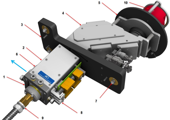
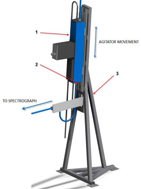
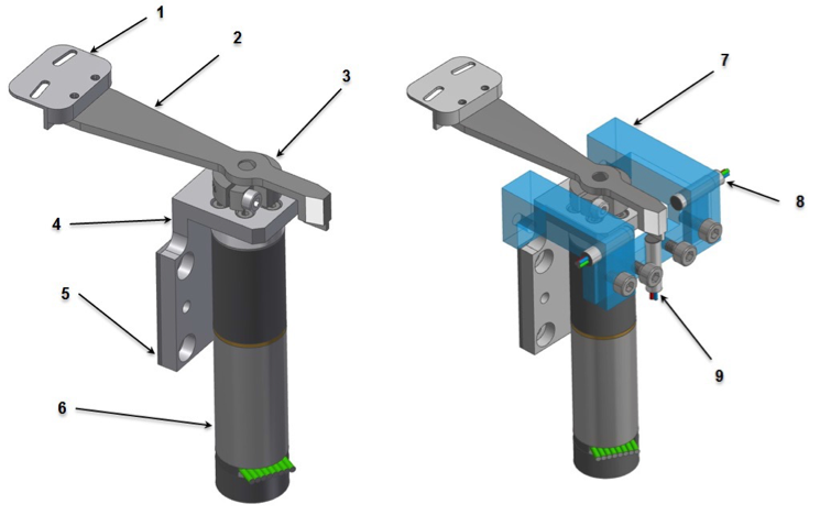
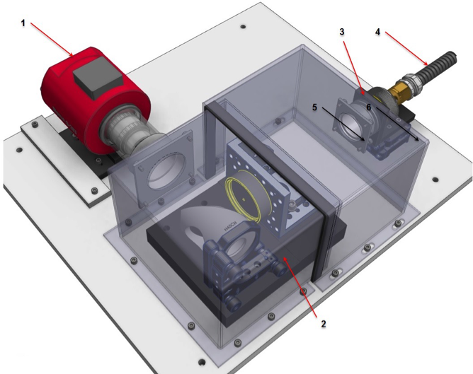
Fibre agitators
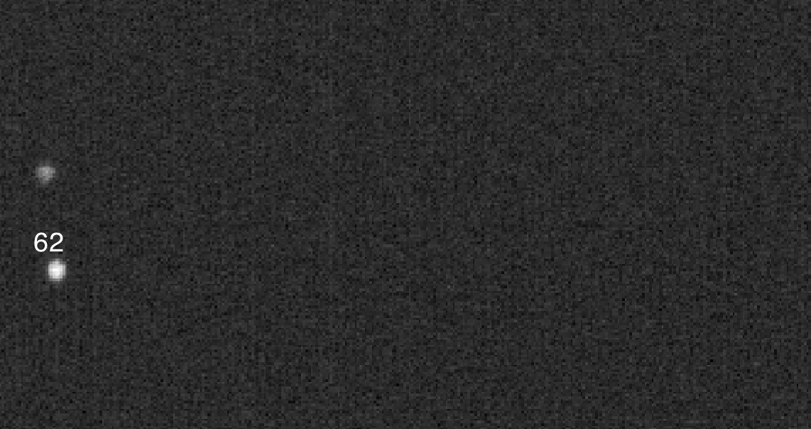
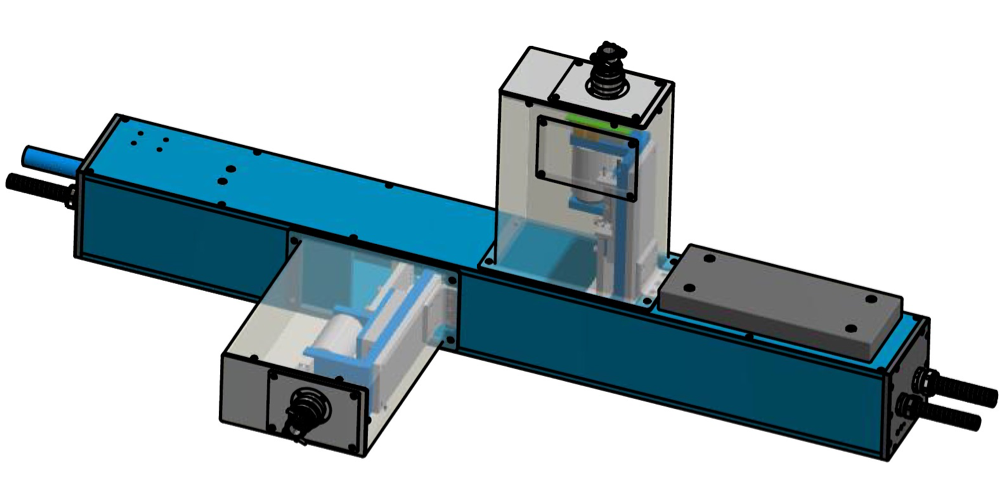
The fiber agitator consists of two orthogonally mounted independent voice coil motor driven mechanisms on a frame through which the optical cable is run in the pier lab before the bench spectrograph, and is seen below. They motors create a sinusoidal pushing motion into fiber bundle (capable of doing so on all 62 fibres), between 5 and 10 mm displacement, running at 1 Hz. The agitators are used in High Resolution modes, to remove modal noise.
While the spectrograph can achieve SNR in excess of 500 without the fibre agitators enabled, there is a gain in the SNR between 50 to 100 dependent on wavelength when using the agitator, and is recommended to be used only in these scenarios. Note that there is no change in spectral profiles or broadening when using the agitator to when not.
Slit mask
The slit mask represents the only moving component inside the bench. The mask can be moved to the standard-resolution slit is open and high-resolution closed; both slits are closed, the high-resolution slit is open and standard-resolution closed, and both slits open. When both slits are closed, all signal to the spectrograph, will be blocked, i.e. all cameras but the Acquisition and Guiding will not be taking images. Multiple checks were conducted of the slit interchange function, where light from the unused slit is blocked by the slit mask. This is done by placing a bright star on one of the standard resolution IFUs, and then make a high resolution mode observation (or vice-versa)- it was found that there was less than 1% of variation in these images when compared to a bias images taken either preceeding, or after the images, demonstrating that the slit correctly blocks all light, and functions as intended.
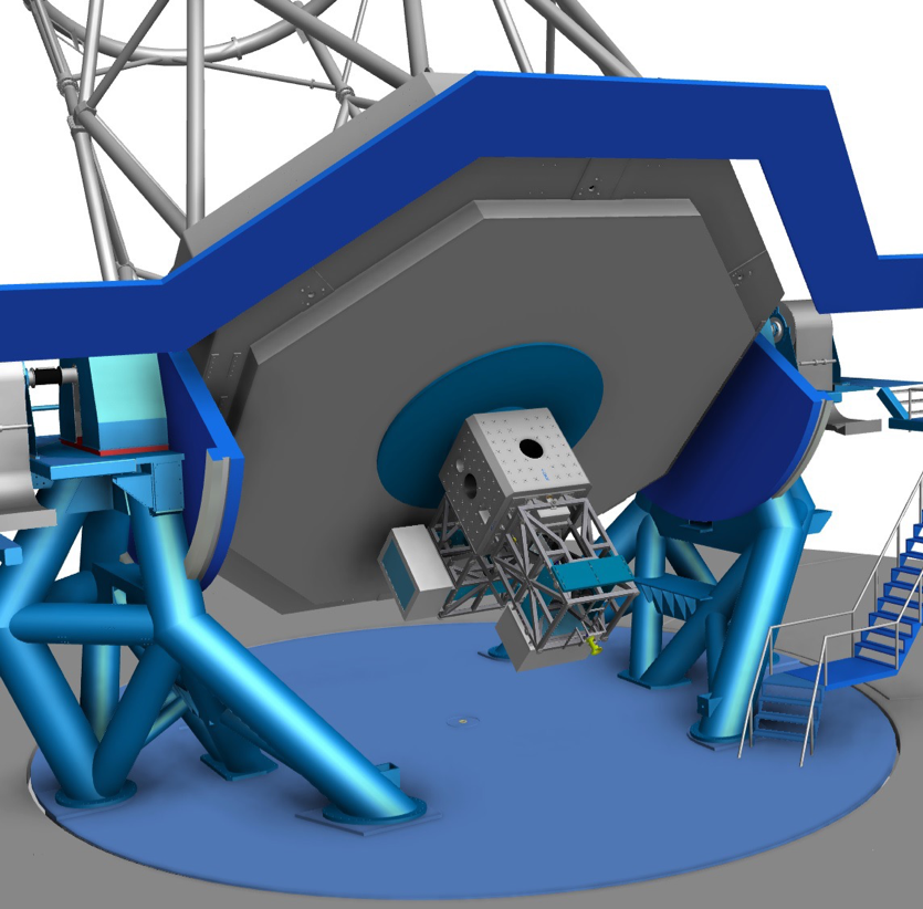
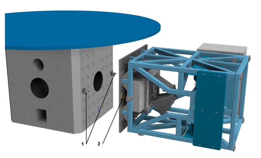
Cassegrain unit components
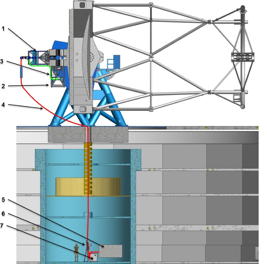
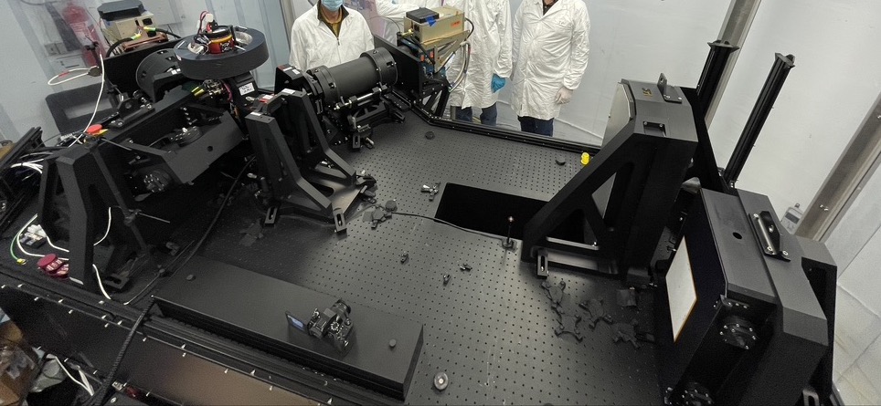
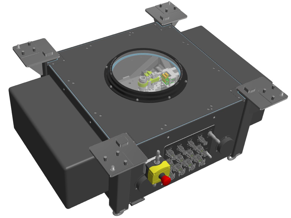
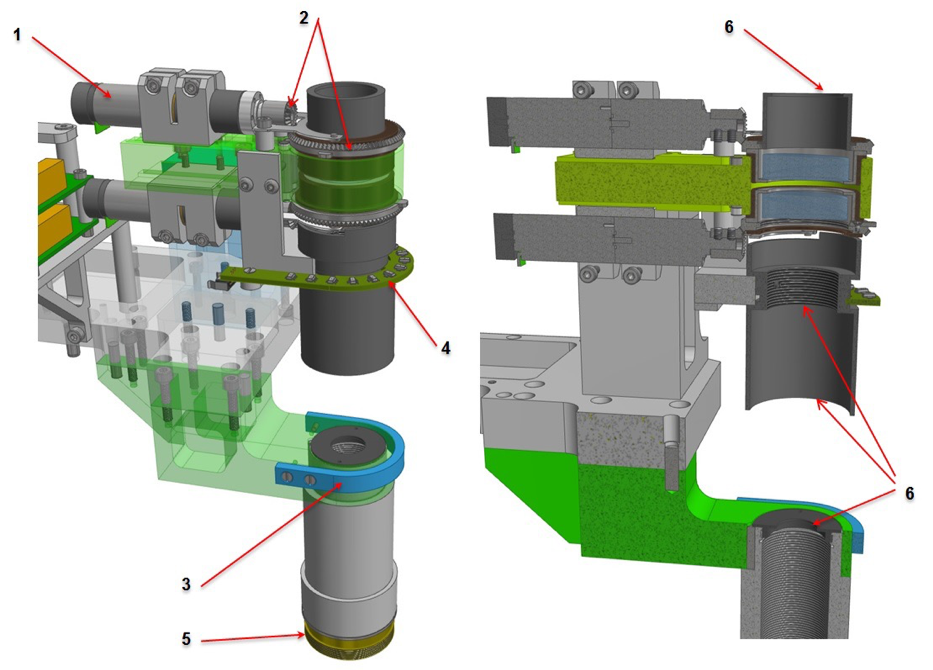
The Cassegrain unit (hereafter cass unit) is mounted on the Cassegrain focus using the Instrument Support Structure. The instrument is usually mounted on the bottom port, to avoid the extra fold mirror reflection when mounted on any of the side ports, which decreases especially the blue sensitivity. Figure 21 below shows the unit mounted on the telescope, and the schematic of the unit before mounting in the lab for visualization. The cass unit consists of three major parts, the telecentric lens, two ADCs, and two IFU probe arms. Here, we only provide the essential details of each for functioning during the night. Further details can be found in the user's manual.
Telecentric lens
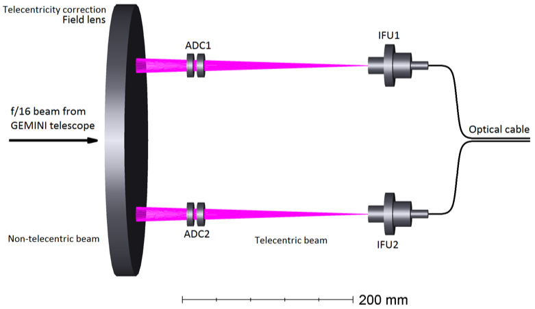
Light arising from the secondary mirror falls off-axis on the fibres. Any correction for this in the IFU unit means reducing the focal length, which in turn means a loss in resolving power. Therefore, a large field lens (32 cm silica lens) correcting for this before light enters the cass unit ensures rays are on-axis to within 1%. The final output displays a plate scale of 1.641±0.001''/mm, and a field of view of ~8.1', with a value of unvigenetted view from the base to a maximum observable radius of 3.67' from the center of the focal plane used for observations. The total field of view used for observations is 7.34'. A f/16 focal length (1625 cm) allows for more tolerance for defocus needed across the focal plane.
Since the field lens and IFU are planar, the images are detected on a plane rather than the actual curved focal surface as expected. There is therefore image broadening due to defocus across the focal plane. It means that if the telescope is focused on an off-axis object, the secondary mirror should move away from the focal surface to bring the object into focus. This can be a significant fraction of the GHOST aperture for objects close to the perimeter of the FoV, wherein images at the edge of the field are not wholly captured by the central microlens, leading to loss of encircled energy. To counteract this across the focal plane of each IFU probe, a defocus correction is applied. This correction is simply calculated using the transformation of a parabolic surface to plane geometry, and is modelled following on-sky testing.
This effects leads to small slit lossses (typically around a few percent) when compared to the centre. From on-sky testing, at a median seeing of 0.7", the seeing at the edge of the IFU focal plane without correcting for defocus varies between 0.8-0.85". Due to this effect, it is preferred that single target objects are observed at the centre of the focal plane whenever possible, and dual targets are best observed at radially symmetric positions from the centre, as this is the best position to correct for defocus.
Atmosphere dispersion correctors
As GHOST is expected to provide a wavelength coverage of 360-900 nm, over an airmass range X, of 1-2, there would exist significant atmospheric dispersion given the variation of seeing over these ranges, scaling approximately to X0.6, and λ-0.2.
Therefore, each individual IFU unit, is equipped with an individual ADC (the field lens ensuring an ideal incidence angle as described earlier), through which light passes before it reaches each IFU. Each ADC provides dispersion correction up to a maximum ZD of 60°, which is suitable for the large wavelength range, and expected airmass limit for most observations (X 2). For corrections at airmasses greater than that, the correction value used is at X of 2.
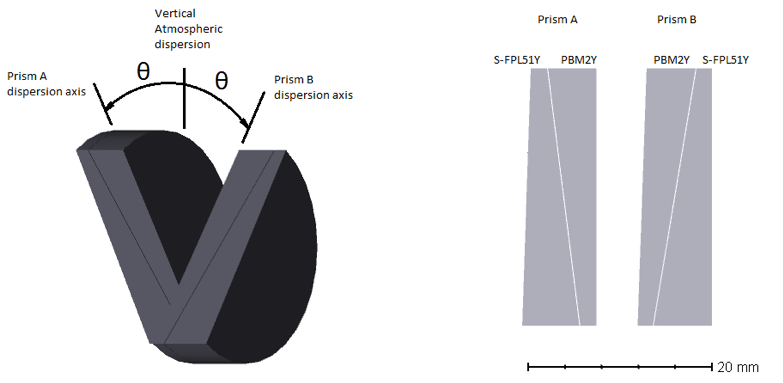
The ADCs are two counter-rotating Risley prisms, where each prism consists of two elements using glasses of different dispersion. When combined, both can be rotated independently to any angle about the beam axis. When orientated in the same direction, their dispersions add and coincide with the direction of atmospheric dispersion (i.e., ADC angle, θ=0), the system is set for maximum Zenith distance (ZD; which is 60°.); while at the maximum value θ of 90°, the system is set for the zenith. The control system can set particular rotation angles for the two prisms to suit any intermediate ZD, and parallactic angle. The small size means glass thickness and light losses are lower while providing a better correction. The prisms were manufactured (Manufacturer: Precision Optical, Prism material used:OHARA i-line glasses, PBM2Y, S-FPL51Y, having refractive index of 1.62 and 1.5 repsectively) with a broadband coating to reduce reflection (of order 1.5%) and increase transmission, and those used have refractive indices suitable for the atmosphere at Cerro Pachon, which do not provide similar corrections at higher altitudes. Sol-gel coatings provide simple and efficient anti-reflection coatings on large, irregularly shaped or delicate component in the IFU. Finally, the angle is given by cos(θ)= tan(ZD)/√3, but additional terms are included for ambient temperature and pressure by the correction software, and are recorded in the FITS Header with the keywords ADCNN, with NN referring to the number of the ADC, and the prism respectively.
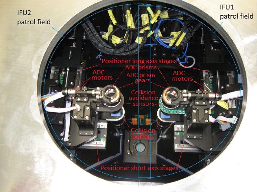
Integral field unit probe arms
The final light capture is done by the IFU situated inside each probe arm, which represents the ultimate aperture. This consists of two robotic arm positioners, which can each probe a hemisphere of 3.7', totaling a total field of view of ~7.4'. Arm 1 contains one standard-resolution IFU unit (hereafter SRIFU1), one standard-resolution sky IFU unit, and one high-resolution IFU unit (HRIFU). Arm 2 contains one standard-resolution IFU unit (SRIFU2), and one high-resolution sky IFU unit. The distribution of the two IFUs in each probe arm is given in the following paragraphs.
The maximum distance the two probe arms can come within each other is 102'', and it is advised for all purposes not to observe targets within 110'', to ensure slight minimal changes in coordinates when guiding, or in proper motions, do not activate collision error. In general, software precludes a collision by identifying a case of a potential collision and issues a warning, both in the Observing tool, and in the instrument software. In case a probe arm is moving within 102'' of another, a collision-avoiding mechanism is triggered on the basis of the Hall effect, which necessitates manual intervention to fix, and the instrument cannot be operated. Finally, if the probes collide for any reason physically, there exists a hard buffer bracket around the IFU assembly to impact much of the stress (between 1000 and 4500 N) depending on the direction and inclination of the collision.
The two standard-resolution IFU units are each composed of seven hexagonal individual microlenses crafted by JenOptik. The apothem of each individual microlens at standard resolution metrologically measured is 0.12 mm, subtending 0.4'' across the flat to flat on sky. The combined light collecting area of each standard resolution IFU is therefore 0.939arcsec2. Filling factor losses as quoted by the manufacturer are 3-6%, but from testing, are more around 7% for the SR IFU, and approximately 15% for the HR IFU. The image of the IFU is sliced into each microlens at pseudo-slit before entering the spectrograph, increasing the resolution by a factor of 3 in the standard-resolution case, as seen below. The dedicate sky IFU of the standard resolution mode subtends 0.4arcsec2.
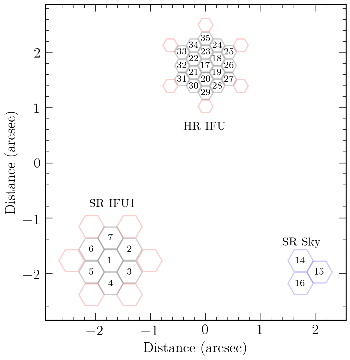
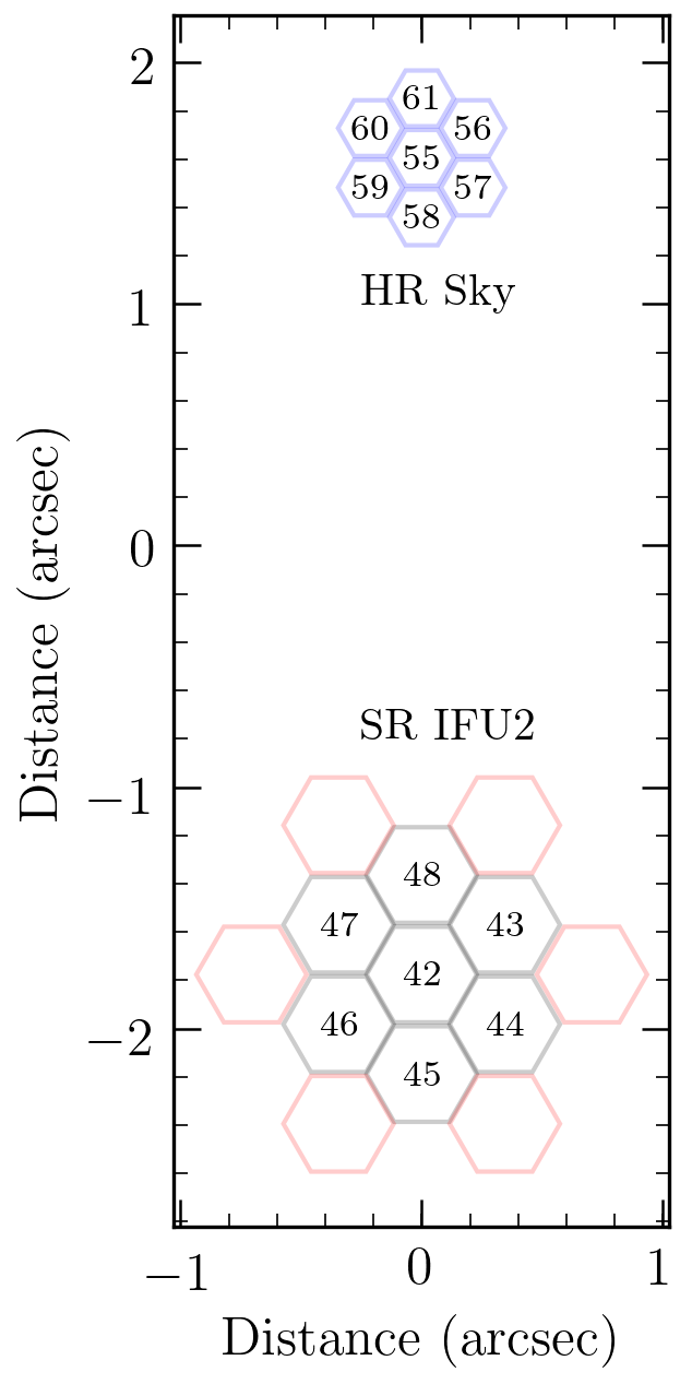
The high-resolution IFU is composed 19 microlenses, hexagonally arranged with similar filling factors. The apothem of each individual microlens is 0.072mm. This results in a subtended total area on the sky of 0.92arcsec2, and represents the aperture. The high resolution sky IFU covers 0.34arcsec2. The final microlens image is sliced by a factor of 5 before entering the spectrograph as a pseudo-slit. The geometrical configuration of both the IFUs is given. The complete unit can be rotated at any position angle to reach a suitable guide star, and is measured North through East.
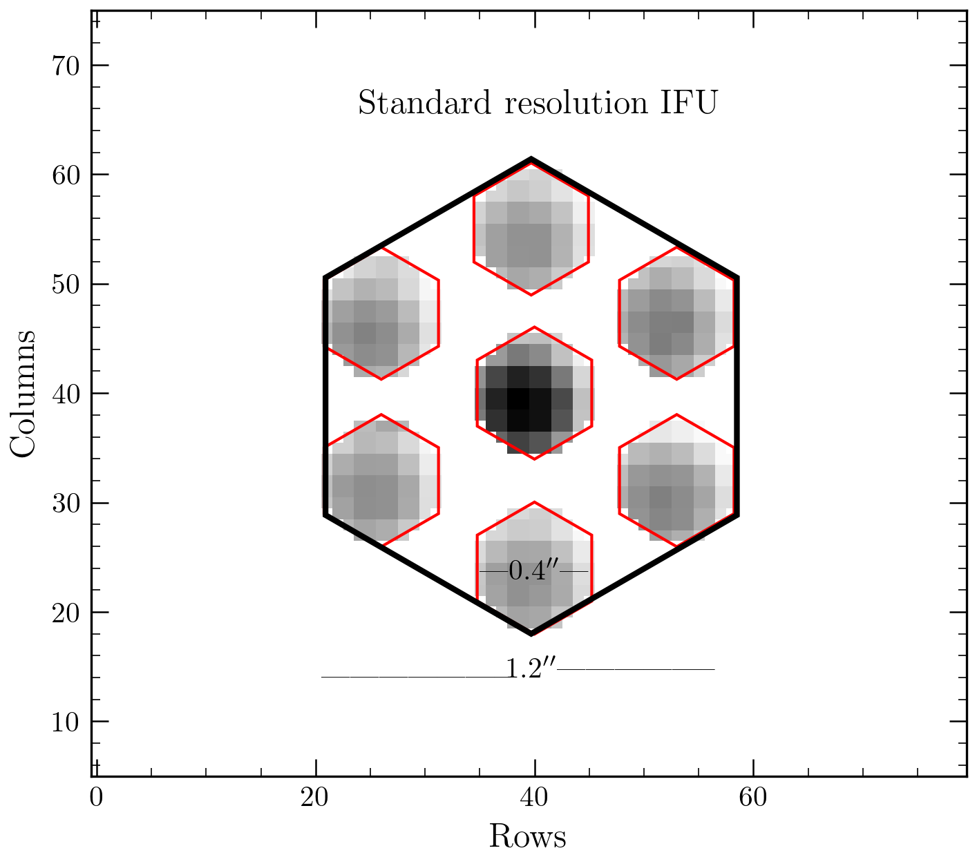
Although the maximum light collecting surface area is 0.9arcsec2 for SR IFU, this is not uniformly circular. Along the short axis, the width is 0.9'', and the long axis 1.2'' is subtended on the sky. Remember, the maximum resolution achievable is 0.4'' in the SR IFU case, and in the HR IFU of 0.24'', i.e. the width of one microlens, and represents the maximum achievable angular resolution on the sky. The total angular resolution is not a linear continuous increase, but rather a discrete value given by the area subtended by each microlens. Finally, although the slit can be approximated to be circular, slit losses due to not observing at the parallactic angle can be considered in cases of moderate seeing depending on each science target, but are corrected using the ADC. The loss of transmission due to the decrease in seeing is given by the slit loss function, as approximated by the standard error function.
Each IFU is not at the centre of the probe arm, i.e. that each separate IFU has a small focus offset from the centre of each probe arm. The IFUs are offset from the centre of the probe arm by a maximum of 1.5 mm, with SRIFU1 and SRIFU2 offset from the centre of their respective probe arms by around 1 mm. For each IFU, an individual focus offset can be added. The focus for each IFU is measured using the reconstructed image, which calculates the image quality as measured from the slit viewing image in the blue and red (this value is scaled to the V-band for the purposes of determining the image quality during observations), which is used to populate the focus offset calculations.
Acquisiton and guide unit
There is no on-instrument wavefront sensor. A series of guide fibres, shown for each science IFU earlier in the IFU schematic, using the same science microlenses, are located around them to provide fine guiding, and direct acqusition. In general, there must be a Peripereal wave front sensor guide star within 6.75' for two IFUs, (and for a single target within 9.85'). This is used to acquire the base position of the focal plane, and centre the science IFUs. The probe mapping is currently precise enough that most targets, across the focal plane are captured in both IFUs within pointing errors of the P2WFS (0.2").
The guide fibers of the instrument are used to center before an exposure, correcting for small probe-map errors, or flexure with the telescope guiding. This guiding, along with P2WFS is monitored over the duration of the exposure, providing small corrections to the positioners to keep IFU well centered. Additionally, the count values provide an independent estimate of the variation of atmospheric conditions near the positioner. In principle, direct acquisition and guiding is possible for targets upto 17 magnitudes in CC70 conditions, and 14 magnitudes in CCAny conditions. The direct acquistion time is a function of the target magnitude, and is given in the following figure. Instrument guiding also allows to acquire targets using a blind offset to accuracies less than 0.1', with targets away by at least 15'', provide both targets have the same base, position angle and P2WFS guide star.
Fibre cable
The optical fibre cable runs from the cassegrain unit, terminating at either the guiding or science slits and the calibration port. It is made of 62 individual fibers, and is a polymicro FBP53/74/94P (53µm core, 94µm polyimide buffer), packed into 8 furcation tubes. The fibres are held inside the tubes using friction, with one to twelve fibers in each of the individual tubes. It includes a switch, to halt all telescope motions if the cable becomes overstressed. The fibers do not come in direct contact with any surfaces. Scrambling is achieved by mechanical agitation in two orthogonal directions, with frequency of 1 Hz using a dedicated agitator.
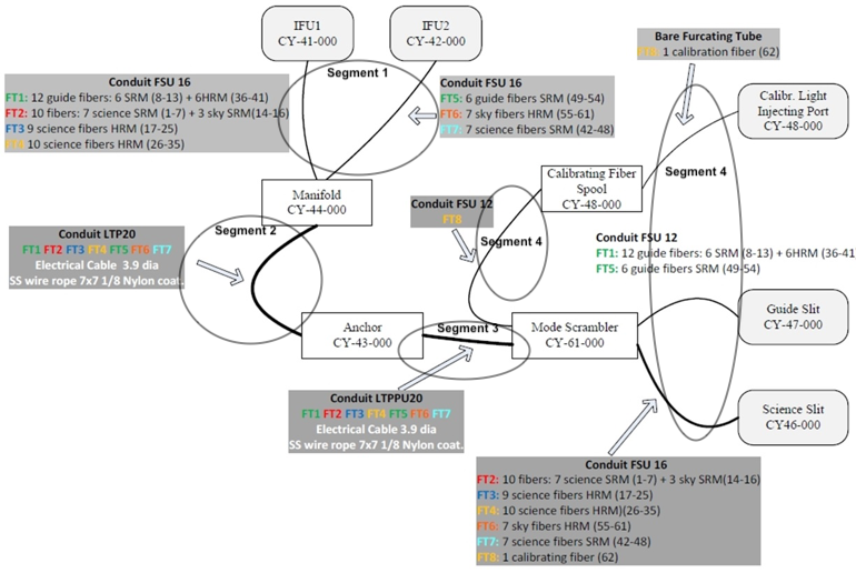
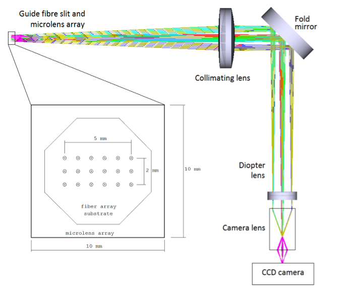
The optical cable ends either at the cassegrain unit, or the slit, or A&G unit. Each fiber array contain the series of holes lithographically etched in the silicon substrate. The geometry of the arrays is identical to the configuration of the corresponding microlens arrays. The center of each microlens coincides with the center of the hole for the insertion of the fiber. The buffer of the fiber is removed over the length required for the fiber array assembly.
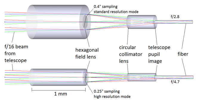
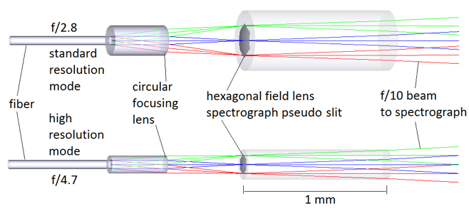
Each fiber feed consists of a pair of microlens arrays that are designed to reimage the secondary mirror onto the fiber core telecentrically. The first lenslet array is located in the telescope focal plane. With its hexagonal aperture, the lens segments the telescope image, and determines the spatial sampling of the fiber input. The second circular lens of the injection optics collimates the flux from different field positions, and, in so doing, images the telescope pupil on to the fiber core in parallel light. The pupil diameter is 50µm for both resolution modes. The optical prescription for the injection optics is the same for both modes, except for the aperture size. As a result, the standard- resolution mode propagates through the fiber at f/2.8, whereas the high-resolution mode is proportionally slower at f/4.7.